CHANGE IN ORGANIC CARBON CONTENT AND YIELD ATTRIBUTES OF POTATO (SOLANUM TUBEROSUM) THROUGH THE APPLICATION OF DIFFERENT LEAF LITTERS

(1)

www.wjpr.net Vol 6, Issue 1, 2017. ₆₅₅

CHANGE IN ORGANIC CARBON CONTENT AND YIELD

ATTRIBUTES OF POTATO (

SOLANUM TUBEROSUM

) THROUGH

THE APPLICATION OF DIFFERENT LEAF LITTERS.

Brij Mohan Singh1 Chandra Mohan Rajoriya2 Mohd Yousuf Mir3 Rajveer Singh

Rawat4 and Dr. Bhanwar Lal Jat5*

1

Department of Botany, SPC Govt PG College Ajmer, Rajasthan, India.

2

Research Scholar, Department of Geography, MDS University, Ajmer, Rajasthan, India.

3

Department of Botany, Bhagwant University Ajmer, Rajasthan, India.

4

RV Book Company, Ajmer, Rajasthan, India.

5

*Department of Agriculture Biotechnology, Bhagwant University Ajmer, Rajasthan,

India.

ABSTRACT

Carbon has become crucial from view point of atmosphere as well as

lithosphere. The largest exchange of carbon take place between

atmosphere and the vegetation, since about half the carbon fixed by

plants is respired back and the net primary production is only about 60

Pg C/ha /year. The global pool of carbon is described in the following

figures. In soil although soil carbon is not directly related to the plant

nutrition yet the plant nutrition is governed by the C status of soil. It

plays pivotal roles in several processes of the soil ecosystem including

nutrient cycling, soil structure, formation, C-sequestration, water

retention detoxification of anthropogenic chemicals and energy supply

to soil microorganisms. The nature, content composition and behaviour of organic matter

in soil are fundamentally important for growth of crops under diverse climat ic

conditions. The organic matter applied to soil is s ubjected to decomposition

depending on the soil and environmental conditions. The experiment was laid out in a

randomized Block Design. As regards to the treatments three levels each of Chinar, Juglens, Morus,

poplar and Salix leaves were employed in C5, C10 and C20; J5, J10 and J20; M5, M10 and

M20; and P5, P10 and P20 and S5,S10 and S20 respectively. The total number of

Volume 6, Issue 1, 655-676. Research Article ISSN 2277– 7105

*Corresponding Author

Dr. Bhanwar Lal Jat

Department of Agriculture

Biotechnology, Bhagwant

University Ajmer,

Rajasthan, India. Article Received on 21 Nov. 2016,

Revised on 11 Dec. 2016, Accepted on 31 Dec. 2016

(2)

www.wjpr.net Vol 6, Issue 1, 2017. ₆₅₆ Bhanwar et al. World Journal of Pharmaceutical Research

combinations worked out to 16 increasing control. The crop was harvested on 28-10-2015. The crop

stands very good. The stems were thick and the plants grew to a height of over 86.80cm.

KEYWORDS: Agro-forestry, Solanum, Carbon, Leaf, ppm.

INTRODUCTION

Environment has different meanings for different people. Most definitions include the physical,

chemical and biological components that influence the life of an organism, Etymologically the

term environment means surroundings Therefore environment can simply be defined as

ones surroundings; which includes everything around the organisms i.e. biotic and Abiotic

components (P.D. Sharma, 2009). The global environment consists of three segments, viz,

atmosphere, hydrosphere and lithosphere. Geologically speaking, the lithosphere is the top crust on

the earth on which the continents and oceans basins rest. It is thickest in the continental region

where it has an average thickness of 40km and thinnest in the oceans where it may have a

maximum thickness of 10 to 12 km. But environmental science is interested only in the upper

few feets of the soil. This soil is not simply one thing but made up of several components

which all together make soil complex. The soil solution contains almost all the essential minerals as

carbonates sulphates, nitrates chlorides and organic salts of Ca, Mg, Na, K etc. are found

dissolved in water (S. Deswal and A. Deswal, 2009). Carbon in soil is found in both organic

and inorganic forms. In most soils the majority of C is held as soil organic carbon (SOC).

Soils are the largest carbon reservoirs of the terrestrial carbon cycle. Soil if managed

properly, can serve as a sink for atmospheric carbon dioxide. Worldwide about 1500 Pg carbon

is stored in first 30 cm o f so il (Batjes, 1996), for India it is o nly 9 Pg

(Bhattacharya et al., 2000) soils contain 3.5% of the earth's carbon reserves, compared with

1.7% in the atmosphere, 8.9% in fossil fuels, 1.0% in biota and 84.9% in oceans (Lal, 1995).

Carbon has become crucial from view point of atmosphere as well as lithosphere. The

largest exchange of carbon take place between atmosphere and the vegetation, since about half

the carbon fixed by plants is respired back and the net primary production is only about 60

Pg C/ha /year. The global pool of carbon is described in the following figures. In soil

although soil carbon is not directly related to the plant nutrition yet the plant nutrition is

governed by the C status of soil. It plays pivotal roles in several processes of the soil

ecosystem including nutrient cycling, soil structure, formation, C-sequestration, water

retention detoxification of anthropogenic chemicals and energy supply to soil

(3)

www.wjpr.net Vol 6, Issue 1, 2017. ₆₅₇ are fundamentally important for growth of crops under diverse climat ic condit ions. The

organic matter applied to soil is subjected to decomposition depending on the soil

and environmental conditions. Humic substances formed in soil; act as highly reactive

natural polymers. Fundamental groups in humic substances also depend on the agro-climatic

conditions (Walker et aL, 2004). Dynamic characteristics such as microbial biomass, soil enzymes

and soil respiration respond more quickly to the changes in crop management practices and type of

cultivation than physio-chemical properties of soils (Chander et al., 1997 and Batra, 2004). The

ancient agriculture is an outcome of dynamic developments since generations that gradually replaced the

organic forming possibly all over the world. The time for this change was different for different countries

and regions. As a result, decline or stagnation in crop yields is reported from one part or the other

including India even with adoption of the recommended technologies (Bhandari et al., 2002 and

Ladha, 2003). The major factors affecting the loss and restoration of soil organic carbon include land

use change, management practices, like cropping intensity, reduced or no tillage, fertilizer and manure

application (Sommerfeld et al., 1988). Labile carbon pool of carbon is the fraction of SOC that

has the most rapid turnover rates and therefore, its oxidation drives the fluex of carbon

dioxide from soils to atmosphere. Also the labile carbon pool is one which is readily

decomposable, easily oxidizable and susceptible to microbial attack and is sensitive to

management induced changes in soil organic carbon. This pool fuels the soil food web and

greatly influences the nutrient cycling for maintaining the quality of soil and its productivity

(Mujumder, 2006). Recent studies have shown that the temperature sensitivity for resistance

organic matter pools does not differ significantly from that of labile pool and that both types of

both will therefore respond similarly to global warming (Fang et al., 2005). Agro-ecosystems play

a central role in the global C cycle and contain approximately 12% of the world terrestrial C.

The terrestrial (plant and soil) C is estimated at 2000 ± 500 Pg which represents 25% of global

C stocks (DOE, 1999). The sink option for CO2 mitigation is based on the assumption that this

figure can be significantly increased if various biomasses are judiciously and/or manipulat ed.

It is clear t hat forests have tremendous potent ia l for C sequestration (1-3 Pg year1)

so as to reduce GHG concentrations in the atmosphere. In this connection agro-forestry systems

will have a great impact on the flux and long-term storage of C in the terrestrial biosphere (Dixon,

1995) as the area of the world under agro-forestry will increase substantially in the near future

undoubtly. The amount of C sequestered largely depends on the agro forestry system put in place,

the structure and function of which are, to a great extent, determined by environmental and

socio-economic factors. Other factors influencing carbon storage in agro-forestry systems include tree

(4)

www.wjpr.net Vol 6, Issue 1, 2017. ₆₅₈ Bhanwar et al. World Journal of Pharmaceutical Research

under solanaceae family. Brinjal is a herbaceous plant growing to 1-3 m in height with woody stem.

Brinjal is a moderately tolerant crop to a wide pH range. A pH of 5.5 -6.8 is preferred.

Though brinjal plants do well in more acidic soils with adequate nutrient supply and

availability. brinjal is moderately tolerant to acid soil that is pH of 5-5. The soils with proper water

holding capacity, aeration, free from salts are selected for cultivation. Soils extremely high

in organic matter are not recommended due to high moisture content of this media

and nutrient deficiencies. But as always, the addition of organic matter to mineral soils will

increase yield. All crops including brinjal absorb carbon dioxide during growth and release it

after harvest. The goal of agricultural carbon removal is to use the crop and its relation to the carbon

cycle to permanently sequester carbon within the soil. This is done by selecting farming methods that

return biomass to the soil and enhance the conditions in which the carbon within the plant will be

reduced to its elemental nature and store in a stable state agricultural sequestration practices

may have positive effects on the soil, air, water and expand food production. On degraded

croplands, an increase of 1 ton of soil carbon pool may increase crop yield by 20 to 40 kilograms

perhectare (Usman et al.2003) Keeping in view the aspects, present investigations entitled "Change in

organic carbon content and yield attributes of potato (lpomoea Batitus) through the application of

different leaf litters", is therefore under taken with the following objectives:- (i) To evaluate the

effect of leaf litters on the yield of brinjal crop. (ii) To analyse the effect of leaf litters on organic

carbon, labile and water soluble carbon in soil.

MATERIALS AND METHODS

This chapter deals with the details of the experiment and the other points dealt with to a briefer degree

are the experimental site, laboratory analysis, the climate and cropping history of the field. The

experiment was conducted during the Kharief season of 2015. The seeds were sown on April 2015.

Experimental site

The present investigation entitled "Response on carbon pools and yield attributes of brinjal (solinum

malongena) crop through application of different leaf litter", was conducted in the village of Batapora

District, Budgam. Jammu and Kashmir.

Climate and weather conditions

Kashmir is situated at an elevation of 6070 ft from sea level at 34.5°N and 74.49°E longitude. This

region has a moderate climate with both the extremes to temperature i.e. summer and winter. In the

winter temperature sometimes falls very low up to -5°C in December-January and hot in summer

(5)

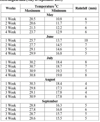
www.wjpr.net Vol 6, Issue 1, 2017. ₆₅₉ 28 inches. The average weekly rainfall, minimum and maximum temperature recorded during

[image:5.595.132.464.135.539.2]

experimental period is given in table 3.1.

Table 3.1: Meteorological data (May to September 2015)

Characteristics of soil

In this region soil is mostly alluvial in nature with low clay and high sand percentage. Soil sample

were collected with the help of soil agar from the experimental site at a depth of 15-20 cm. The soil

sample which was then analysed at Department of soil Science, Share Kashmir University of

agriculture science and technology (Kashmir).

Table 3.2 Physio chemical properties of soil.

S. No. Particulars Value

1. pH 7.7

2. Available organic carbon 0.47

3. Sand 60%

4. Clay 14%

Weeks Temperature

0

C

Rainfall (mm)

Maximum Minimum

May

1 Week 20.5 10.8 6

2 Week 20.6 11.7 7

3 Week 21.3 12.2 6

4 Week 23.7 12.9 6

June

1 Week 25.7 13.7 10

2 Week 27.7 14.5 7

3 Week 29.1 14.6 5

4 Week 29.9 16.8 5

July

1 Week 30.2 18.4 8

2 Week 30.7 18.7 7

3 Week 30.9 19.3 5

4 Week 30.8 19.0 8

August

1 Week 30.3 18.4 4

2 Week 29.8 17.3 4

3 Week 29.1 17.8 4

4 Week 30.9 17.8 6

September

1 Week 28.8 16.3 5

2 Week 27.8 16.8 6

3 Week 28.7 15.7 5

(6)

www.wjpr.net Vol 6, Issue 1, 2017. ₆₆₀ Bhanwar et al. World Journal of Pharmaceutical Research

5. Slit 26

6. Soil texture Sandy

loam

Experimental details

Design and treatment Levels of Chinar leaves

Levels of Juglens leaves

Levels of M orus leaves

Levels of Poplar leaves

Levels of Salix leaves

C5 = 5 tone of Chinar

leaves per hectare

J5 =5 tone of

Juglens leaves per hectare

M5 = 5 tone of Morus

leaves per hectare

P5=5 tone of Poplar

leaves per hectare

T5=5 tone of Salix

leaves per hectare

C10 = 10 tones of

Chinar leaves per hectare

J 10 = 10 tone of

M10= 10 tone of

Morus leaves per hectare

P10=10 tone of Poplar

leaves per hectare

T10=10 tone of Salix

leaves per hectare

C20 = 20 tones of

Chinar leaves per hectare

J20=20 tones of

M20 = 20 tone of

Morus leaves per hectare

P20=20 tone of Poplar

leaves per hectare

T20 = 20 tones of Salix leaves per hectare

Treatment Combinations

T1 = C5 T2 = C10 T3 = C20 T4 = J5 T5 = J10 T6 = J20 T7= M5 T8 = M10

T9 = M20 T10 = P5 T11 = P10 T12 = P20 T13 = S5 T14 =

S10 T15 =S20

T16= Control

Details of crop cultivation Crop= Brinjal (Solarium

melongena) Spacing= Row to row - 50 cm Plant to plant - 50 cm

Variety= Zaith Vangan (vernicular) Duration of crop =180 day Design of experiments = (3 x 3 factorial) R.B.D

Dimension details Total number of

treatments:-16 Total number of replications:-3 Total number of plots:-48

Individual plot size:-1.5 x 1.5

Area of each plot:- 2.25 m2

Length of experimental field:- 29.1m

Width of experimental field:-

7.3m Width of bund:- 0.3m

Width of sub-irrigation channel:-0.5m Net cultivated area:- 108.m2 Gross area:- 212.48m2

Analysis of variance (ANOVA)

Analysis of treatment for all the treatment in Randomized Block Design was carried out. For

testing the hypothesis the following ANOVA table was used.

Table: 3.3 Skeleton of ANOVA

Source of

variation d. f. S.S. M.S.S F. Cal

F (Table) at Result 5% Due to

replication (r-1) R.S.S.

R.S.S. r-1

(7)

www.wjpr.net Vol 6, Issue 1, 2017. ₆₆₁ Due to

treatment (t-1) T.S.S.

T.S.S. t-1

M.T.S.S.

M.E.S.S. (r-1) (t-1)

Due to error (r-1) (t-1) E.S.S. E.S.S. (r-1) (t-1)

E.S.S. M.E.S.S.

F (t-1) (r-)(t-1)

Total (rt-1) T.S.S. - - -

Where:- d. f. = Degree of

freedom t = Treatment M.S.S.= Mean Sum Square

r = Replication R.S.S.= Replication Sum Square T.S.S.=Total Sum Square

S.S.= Sum of Square M.R.S.S.= Mean Replication Sum

Square M.T.S.S.= Mean Treatment Sum Square

E.S.S.= Error Sum Square M.E.S.S.= S.E. (d) x ‘t’ error d.f. at 5% level of significance S.E. (d) = 2 x M.E.S.S.

r

The significance and non- significance of the treatment effect was judged with the help of 'F'

variance ratio test. Calculated 'F' value was compared with the table value of 'F' at 5% level of

significance. If the calculated value exceeds the table value, the effect was considered to be

significant. The significant differences between the means were tested against the critical

differences at 5% level of significance. For testing the hypothesis, the ANOVA table was used.

Cultural Operations:-The package of cultural operations used in raising the crop is

described below:

Land preparation:-The field was prepared by one plough using soil turning plough,

harrowed and finally planked for leveling, thereafter field was laid out in plots and all

grasses stables and weeds were picked up from field.

Application of leaf litter:- Leaves were applied to the various plots according to the

treatment schedule. The amount of leaves actually applied is given in table.

Table: 3.4. Rate of application of leaf litter

Source Rate of application Amount of leaves/plot

Chinar leaves

5 t/ha 10 t/ha 20 t/ha

0.75 kg 1.5 kg 3.0 kg

Juglens leaves

0.75 kg 1.5 kg 3.0 kg

Morus leaves

(8)

www.wjpr.net Vol 6, Issue 1, 2017. ₆₆₂

Bhanwar et al. World Journal of Pharmaceutical Research

1

Poplar leaves

0.75 kg 1.5 kg 3.0 kg

Salix leaves

0.75 kg 1.5 kg 3.0 kg

Irrigation

After the application and mixing of leaves field was irrigated through the main and two

sub-irrigation channels. The sub-irrigation breaks hard soil and make field ready for transplantation.

Transplanting of seedlings

The thirty days old seedlings of brinjal were transplanted in the main research plot. This

operation was done on 01-05-2015. The planting was done on pre-marked spacing (50cm

x 50cm).

Inter culture

Inter culture with the help of the inter culture equipment was done at 30 DAT, weeding was

not found to be necessary but inter culture was felt would help in the aeration of the root.

Application of fertilizers:- The recommended fertilizers for brinjal (Solanum

malongena) given below:-

The three fertilizers urea, DAP and MOP were mixed and accordingly applied to each

plot. Urea (150kg/ha) DAP (80kg/ha) and MOP (60kg/ha) that is 33.75g, 18.0g and 13.5g per

plot respectively.

Table-3.5- Crop calendar

S. No. Date Operation

1. 20.04.2015 Ploughing

2. 21.04.2015 Harrowing and planking 3. 22.04.2015 Bunds and furrow made 4. 23.04.2015 Layout of design

5. 24.04.2015 Application of leaves 6. 25.04.2015 First irrigation 7. 01.05.2015 Transplantation

8. 02.05.2015 Second irrigation(after transplantation) 9. 02.06.2015 Interculture

10. 10.06.2015 Fertilizer application

(9)

www.wjpr.net Vol 6, Issue 1, 2017. ₆₆₃ OBSERVATION

The observation record are classified as per and post-harvest observation. The observation

were record at the following stages:- (i) Plant height (90 DAT) (ii) Number of Branches (90

DAT) (iii) Number of fruits per plant (95-165 DAT) (iv) Yield per plant (100-180 DAT) (v)

Yield per plot (100-180 DAT).

Pre-harvest observations:- (i) Plant height: The plant height in centimeters was recorded 90 DAT. Plant

height was recorded from the base to the tip of the plant. Three plants randomly selected from the

observational plot were used for measuring plant height. (ii) Number of branches: Number of branches

was recorded 90 DAT. Three plants randomly selected from the observational plot were used for the

number of primary and secondary branches. (iii) Number of fruits per plant:-Number of fruits per

plant was observed from 95-165 DAT. Five plants randomly selected from the observational plot

was used for finding the number of fruits per plot. (iv) Y ie ld p e r p la nt:-Yield per plant was

observed from 100-180 DAT. Three plants randomly selected from the observational plot were

used for observing yield per plant. The yield of these three randomly selected plants have been

added and divided by three which gives the average yield of each plant in the observing plot. (v)

Y i e l d p e r p lo t : - The average yield observed per plant in any observation slap lot was

multiplied by the total number of plants in a plot gives the total yield of that observational plot. It

was observed from 100-180 DAT.

Post-harvest observations:- The post-harvest observations included soil analysis for the percentage of

organic carbon, labile carbon and water soluble carbon.

Determination of organic carbon:- Organic carbon in soil was determined by using Walkley

Black Method (1956).

Procedure:- Take 1 g of soil sample, passed through a 0.5 mm non-furrows sieve in a 500 ml

conical flask. Add 10 ml of 1N k2Cr207 and mix the soil in the solution by gently swirling the

flask. Add 20 ml of conc. H2SO4 and mix it by gentle rotation for about one minute, to ensure

complete reaction of reagent. Allow the flask to stand for about 30 minutes. Run

standardization blank in the same way. Add 20ml of water to the flask to dilute the

suspension. Filter if it is expected that the e nd po int o f t he t it rat io n w ill no t be c le ar.

Ad d 10 ml o f 85 p erce nt orthophosphoric acid (H3PO4), 0.2g of sodium fluoride and

30 drops of diphenylamine indicator. Back titrate the solution with standard furrows

(10)

www.wjpr.net Vol 6, Issue 1, 2017. ₆₆₄ Bhanwar et al. World Journal of Pharmaceutical Research

blue as the titration proceeds. At the end point this colour sharply shifts to a brilliant green

giving one drop end point. If the sample has consumed over 10 ml of potassium dichromate,

the determination is to be repeated with small quantity of sample like 0.2 or 0.5g.

Calculation:-Percent organic carbon = Me Ox — me Red x 0.003x 100 Wt. of sample x 0.76

Where, me Ox = ml K2Cr207 x NK2cR207, me Red = ml Fe(NH4)2 (SO4)2 x N Fe (NH4) 2(SO4)2

0.003 = me weight of carbon 100 = decimal to percentage conversion factor.

Labile soil carbon:- Labile or permanganate oxidizable soil carbon (PoSc) was determined by

using method of Blair et aL, 1995.

Procedure:- Take 3g of air-dried soil in a 50 ml centrifuge tube. Add 30 ml of 20 molar KMn04

to soil in centrifuge tube and run a blank without taking soil. Shake the contents for 15 minutes

and centrifuge for 5 minutes to 2000 rpm. Transfer 2m aliquot of supernatant into 50 ml

volumetric flask. Read the absorbance at 560565 nM and determine conc. of KMn04 from

standard calibration curve.

Calculation:- Pose (mg kg-1) = (B-S) x 50/2 x Vol. of KMn04"1) x 1000x9

1000 x weight of soil (g)

Where, B = Conc. (M molar) of KMn04 in blank. S = Conc. of (m molar) of KMnO4 in sample 50/2

= Dilution factor 9 = gm C oxidized by (m mole KMnO4).

Water soluble carbon:-The water soluble carbon in soil was determined by using the method of

(McGill, 1986).

Procedure:-Take 10 g soil in a centrifuge tube and add 20 ml distilled water. Shake it for

one hour and centrifuge for 20 minutes at 9000-1000 rpm. Filter the aliquot in a beaker.

Take 10 ml of aliquot in 250 ml conical flask and add 2 ml 0.2N K2Cr207. Then add 10

ml of conc. H2SO4 and 5 ml orthophoric acid and keep the volumetric flask on water bath at

100°C for 30 minutes. Now titrate the contents in flask with 0.01 N FAS, the end point is

green. Also run a blank simultaneously.

Calculation:- W Se (ppm) = 2(B-S)/B*0.2*0.003*20/10*/10*104 Where, B = ml of 0.01 N FAS used

(11)

www.wjpr.net Vol 6, Issue 1, 2017. ₆₆₅ RESULTS AND DISCUSSION

The results obtained during the present study have been presented in this chapter through data, tables

and graphs, whatever necessary. The treatment effect on the characters studied have been

interpreted and discussed in the light of scientific evidence.

Plant height (cm)

There was a significant response to the main treatments and an increase in plant height at all

first and second level of treatments. The maximum increase in plant height due to first level of

treatment (81.07 cm) was found at T1 with 0.75 kg of Chinar leaves. The minimum increase at first

level of treatments (80.03 cm) was found at T4 with 0.75 kg Juglens leaves. The average plant

height at first level of treatment was 80.60 cm. At the second level of treatment maximum

increase in plant height (82.33 cm) was recorded at T2 with 1.5 kg Chinar leaves, and

minimum increase (81.27 cm) at T11 with 1.5 kg poplar leaves. The average plant height

recorded at second level of treatment was 81.73 cm. At the third level of treatment maximum

increase in plant height (86.83 cm) was observed at T9 with 3 kg of morus leaves and minimum

increase (84.70cm) at 115 with 3 kg teak leaves. The average plant height at third level of

treatment observed was 85.53 cm.

Table- 4.1-Effect of leaf litter on plant height (cm) at 90 DAT

Treatment Plant height

R1 R2 R3 MEAN

T1C5 83.4 80.0 79.8 81.07

T2C10 84.6 82.3 80.1 82.33

T3C20 86.8 83.9 80.1 82.33

T4J5 T5J10 T6J20 T7M5 T8M20 T9M20 T10P5 T11P10 T12P20 T13S5 T14S10 T15S20

T0

F-Test S

S.Ed(+-) 1.209

(12)

www.wjpr.net Vol 6, Issue 1, 2017. ₆₆₆ Bhanwar et al. World Journal of Pharmaceutical Research

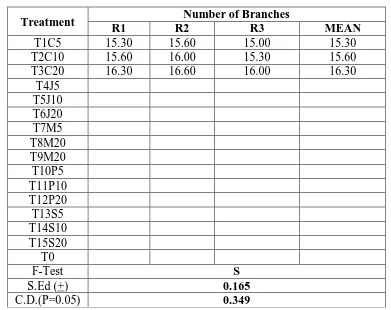
Number of branches

There was a significant response to other main treatments or first and second of treatments on

the number of branches. At first level of treatment the highest number of branches (15.40) was

found at T10 with 0.75 kg poplar leaves and lowest (15.20) at T13 with 0.75 kg salix leaves.

Average number of branches at this level was 15.30. At second level of treatment the

maximum number of branches counted was 15.73 at T5 with 1.5 kg of juglens leaves and

minimum branch counted was 15.50 at T5, T11 and T14 with 1.5kg of morus, poplar and salix

leaves respectively. The average branch number of this stage was 1 5.57. At third level of

treatment the maximum branch number (16.40) was counted at T6 and T9 with 3 kg of

juglans and morus leaves respectively and minimum (16.30) at T3, T12 and T15 with 3

kg of chinar, poplar and salix leaves respectively. The average number of branches at

[image:12.595.101.492.348.658.2]

third level of treatment was 16.34 branches per plant.

Table -4.2-Effect of leaf litter on number at 90 DAT

Treatment Number of Branches

R1 R2 R3 MEAN

T1C5 15.30 15.60 15.00 15.30

T2C10 15.60 16.00 15.30 15.60

T3C20 16.30 16.60 16.00 16.30

T0

F-Test S

S.Ed (+) 0.165

C.D.(P=0.05) 0.349

Number of fruits per plant

There was a significant response to either third or first and second level of treatment. The

maximum number of fruits counted at first level of treatment (37.22) was at T13 with 0.75kg at

T4 with 0.7kg of Juglens leaves. The average fruits counted at this level of treatment were 36.53.

(13)

www.wjpr.net Vol 6, Issue 1, 2017. ₆₆₇ 1.5kg of Salix leaves and minimum (37.77) at T8 with1.5 kg of Morus leaves. The average

number of fruits observed at this level of treatment was 38.30. At the third level of treatment

the maximum number of fruits 45.99 was observed at T15 with 3kg of Salix leaves and

minimum 41.88 at T3 with 3 kg Chinar leaves. The average number of fruits counted at

this level of treatment was 43.72 fruits per plant.

Table 4.3-Effect of leaf litter on number of fruit per plant at 95-165 DAT.

Treatment Number of fruit per plant

R1 R2 R3 MEAN

T1C5 73.33 36.33 36.00 36.55

T2C10 38.66 38.00 38.66 38.44

T3C20 42.66 41.66 41.33 41.88

T0

F-Test S

S.Ed (+) 0.673

C.D.(P=0.05) 1.426

Yield per plant

The yield per plant also increased significantly at all levels of treatment. At first level of treatment the

maximum yield (3.10 kg) was observed at Ti3 treated with 0.75 kg teak leaves and minimum (2.98

kg) was observed at T4 due to 0.75 kg of Chinar leaves with average yield of 3.04 kg. The second

level of treatment had the highest yield 3.24 kg at T4 with 1.5 kg Salix leaves and the lowest

3.15kg at T8 due to 1.5kg of Morus leaves, with an average yield of 3.19 kg per plant.

The maximum yield due to top level of treatment was 3.83kg at T15 treated with 3 kg of

teak leaves and the minimum yield 3.49 kg at T3 treated with 3 kg of teak leaves and the

minimum yield 3.49kg at T3 treated with 3 kg of Morus leaves. The average yield observed at

(14)

[image:14.595.116.483.82.399.2]

www.wjpr.net Vol 6, Issue 1, 2017. ₆₆₈ Bhanwar et al. World Journal of Pharmaceutical Research

Table 4.4-Effect of leaf litter on yield per plant (kg) at 100-180DAT.

Treatment Yield per plant (kg)

R1 R2 R3 MEAN

T1C5 3.11 3.02 3.00 3.05

T2C10 3.21 3.16 3.21 3.20

T3C20 3.55 3.47 3.44 3.49

T0

F-Test S

S.Ed (+) 0.058

C.D.(P=0.05) 0.124

Yield per plot

A moderate high increase in fruit yield per plot was observed at the third level of treatment and also

a significant increase at first and second level of treatment. The maximum yield due to first level of

treatment was 27.79 kg at T13 with 0.75 kg teak leaves and the minimum yield (27.16 kg) at T7

with 0.75 kg morns leaves, with an average yield of 27.37 kg. At the second level of treatment

the maximum yield (29.16kg) was observed at T14 with 1.5kg of teak leaves and the

minimum (28.33 kg) at T8, treated with 1.5 kg of mango leaves, with an average yield of28.71

kg of potato per plot. The maximum yield due to third level of treatment (34.49 kg) at T15 with 3

kg of Salix leaves and the minimum yield (31.41 kg) at T3 due to 3 kg of Chinar leaves. The

average yield per plot at third level of treatment was 32.76 kg per plot. Thus the maximum

yield observed in any plot was 34.49 kg or 15.33 tons per hectare. The decrease from the

average yield (17.50 tons per hectare in India) may be due to temperature variations at Kulgam

Kashmir, as the potatol grows and yields best from 28 to 38°C.

Table 4.5-Effect of leaf litter on yield per plot (kg) at 100-180DAT.

Treatment Yield per plot (kg)

R1 R2 R3 MEAN

T1C5 27.99 27.25 27.00 27.49

(15)

www.wjpr.net Vol 6, Issue 1, 2017. ₆₆₉

T3C20 31.99 31.23 30.99 31.41

T0

F-Test S

S.Ed (+) 0.533

C.D.(P=0.05) 1.131

Yield per hectare(tons)

The of data on yield per hectare at 100-180 DAT was recorded and found Significantly

increment in yield per hectare with increase in dose of leaf litter. The maximum yield (17t) per hectare

was recorded in treatment combination T15S20 comparison to treatment combination T6J20 with

16.50 tons per hectare and minimum yield (13.11t) per hectare was recorded in T0 (control). The

significant difference in yield per hectare was recorded due to variation in organic carbon

present in leaves of different species of trees. Available carbon is the indicator of available nitrogen

in the soil and nitrogen is the major nutrients which support the vegetative growth and yield of plants.

Table 4.6-Effect of leaf litter on yield per hectare (tons) at 100-180DAT.

Treatment Yield per Hectare

R1 R2 R3 MEAN

T1C5 13.82 1342 13.33 13.33

T2C10 14.26 1404 14.26 14.26

T3C20 15.77 1542 15.28 15.28

(16)

www.wjpr.net Vol 6, Issue 1, 2017. ₆₇₀ Bhanwar et al. World Journal of Pharmaceutical Research

T15S20 T0

F-Test S

S.Ed (+) 0.259

C.D.(P=0.05) 0.549

Percent organic carbon

Carbon stored in soils is derived from litter carbon stored in soils is derived from litter and root

inputs, while losses result from microbial degradation of organic matter (OM) and erosion

within limits. Soil C increases with increasing soil water and decreases with increasing

temperature. A significant increase was found due to addition of leaves as they decompose and gets

converted into litter which intern increases the soil organic carbon content. At first level of

treatment the maximum carbon content 0.53% was observed at T7 and T13 due to 0.75 kg of

mows and Salix leaves respectively. At second level of treatment the maximum yield 0.95%was

observed at T8 with 1.5 kg of Morus leaves. The maximum amount of organic carbon in any plot

(0.69%) was due to T15 at third level of treatment with 3 kg of Salix leaves and the lowest

0.51% and 0.48% was observed at T4 and T16 control respectively. The average yield at

[image:16.595.112.482.71.145.2]

first second third level of treatment was 0.52% and 0. 66% respectively.

Table 4.7: Effect of leaf litter on organic carbon after harvesting of crop.

Treatment Percent 0.C

R1 R2 R3 MEAN

T1C5 0.51 0.52 0.54 0.52

T2C10 0.56 0.57 0.58 0.57

T3C20 0.61 0.66 0.65 0.64

T0

F-Test S

S.Ed (+) 0.011

(17)

www.wjpr.net Vol 6, Issue 1, 2017. ₆₇₁ Water soluble organic carbon (ppm)

Water soluble organic carbon (WSOC) accounts only for a small portion of the total organic

carbon in soil. Nevertheless WSOC is considered the most mobile and reactive organic carbon

fraction thereby can control a number of physical, chemical and biological processes in both

aquatic and terrestrial environments. There was a significant increase in WSOC at all the three

levels of the treatment. The maximum amount of WSOC 49.20 ppm was observed at T10 with

0.75 kg of poplar leaves and 56.40ppm at second level of treatment. The highest amount of WSOC

found in any plot 69.60ppm was observed at T3 with 3kg of Chinar leaves. The average amount

of WSOC observed at first, second and third level of treatment was 45.60ppm, 53.36ppm and

[image:17.595.116.480.304.620.2]

67.04 respectively.

Table 4.8: Effect of leaf litter on WSOC after harvesting of crop.

Treatment WSOC (ppm)

R1 R2 R3 MEAN

T1C5 40.80 52.80 39.60 44.40

T2C10 52.80 52.80 52.80 52.80

T3C20 69.60 67.20 72.00 69.50

T0

F-Test S

S.Ed (+) 5.076

C.D.(P=0.05) 10.760

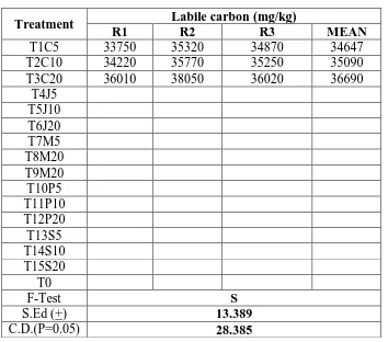
Labile carbon (mg/kg)

By contrast, the labile (bio-available) pool of carbon is primarily influencedby new organic matter

(originating from plants and/or animals) contributed annually. A significant increase in the percent

of labile carbon was seen at all the three levels of the treatment. At first level of treatment the

maximum amount of labile carbon 348.90 mg/kg was found at T10 treated with 0.75 kg poplar

leaves. At second level of treatment the maximum amount of labile carbon 357.63 mg/kg was

(18)

www.wjpr.net Vol 6, Issue 1, 2017. ₆₇₂ Bhanwar et al. World Journal of Pharmaceutical Research

(378.23 mg/kg) was seen at T15 treated with 3 kg of Salix leaves. The minimum amount of

labile carbon (339.80 mg/kg and 303.13 mg/kg) among all plots was seen at T13 and T16

with 0.75kg Salix leaves and control respectively. The average amount of labile carbon at first,

second and third level of treatment was 344.07 mg/kg, 351.88 mg/kg and 371.56 mg/kg.

[image:18.595.123.477.182.494.2]

Table 4.3- Effect of leaf litter on labile carbon after harvest of crop.

Treatment Labile carbon (mg/kg)

R1 R2 R3 MEAN

T1C5 33750 35320 34870 34647

T2C10 34220 35770 35250 35090

T3C20 36010 38050 36020 36690

T0

F-Test S

S.Ed (+) 13.389

C.D.(P=0.05) 28.385

CONCLUSION

The experiment entitled Change in organic carbon content and yield attribute of potato (Solanum

tuberosum) was carried out in the Kharief season of 2015 at the field of district Kulgam Kashmir. The

experiment was laid out in a randomized Block Design. As regards to the treatments three levels each

of Chinar, Juglens, Morus, poplar and Salix leaves were employed in C5, C10 and C20; J5, J10

and J20; M5, M10 and M20; and P5, P10 and P20 and S5,S10 and S20 respectively.

The total number of combinations worked out to 16 increasing control. The crop was harvested on

28-10-2015. The crop stands very good. The stems were thick and the plants grew to a height of over

86.80cm. A brief report of the pre and post-harvest observations are now placed before the reader. (i)

There was a good response of the main treatment (3kg leaves/plot) as well as first (0.75kg

leaves/plot) and second (1.5kg leaves/plot) levels of treatments. (ii) A good response to number of

secondary branches was also seen but not on primary branches. Thus primary and secondary

(19)

www.wjpr.net Vol 6, Issue 1, 2017. ₆₇₃ of treatment of about 1.30 branches. (iii) A maximum number of fruits (45.99) per plant were

observed at T15 with 3 kg teak leaves. (iv) A significant increase in yield of potato was seen at all the

three levels of treatment. A maximum yield of 34.47 kg was observed at T15 with 3kg Salix

leaves. (v) All the three levels of treatment show a significant response towards carbon pools

in soil organic carbon reaches maximum to 0.69% at 115, water soluble carbon maximizes up to

69.60ppm at T3 and labile carbon reaches its maximum 378.23 mg/kg at T15.Chinar, Juglens,

Morus, poplar and Salix leaves at all the three levels were found to effect all the growth, yield

and post-harvest soil parameters. Among the third level treatments Salix leaves alone show good

response on most of the parameters except plant height, number of branches and organic

carbon that were affected by Morus, Juglens and Salix leaves respectively. So it can be

concluded that all these five types of tree leaves (Litter) effect the plant growth, yield as well as

carbon pools in soil.

REFERENCES

1. Batjes, N.H. (1996). Total carbon and nitrogen in the soils of world. European Journal of Soil

Science, 47: 151-163.

2. Batra, L. (2004). Dehydrogenase activity of normal saline and alkaline soils under different

agriculture management systems. Journal of Indian Society of Soil Science, 52(2): 160-163.

3. Berg, B. (2000). Litter decomposition and organic matter turnover in northern forests soils. Forest

Ecology and Management, 133(1-2): (165 p.).

4. Bhattacharyya, T., Pal, D.K., Mandal, C. and Velayutham, M. (2000). Organic carbon stock in

Indian. Soils and their geographical distribution. Cu!. Sci., 79: 655-660.

5. Chander, K., Goya!, S., Mundra, M.C. and Kapoor, K.K. (1997). Organic matter,

microbial biomass sand enzyme activity of soils under different crop rotations in the tropics.

Biology and Fertility of Soils, 24: 306-310.

6. Cotrufo, M.F. De. Santo, A.V. Alfani, A. Bartoli, G. and De, Cristofaro, A. (1995). Effect

of urban heavy metal pollution on organic matter decomposition in Quercus ilex L. woods.

Environmental pollution, 89(1): 81-87.

7. Dinar, M. and Rudics, J. (1985). Effect of heat stress on assimilates partition in tomato. Ann.

Bot., 56: 239-249.

8. Ding Lei, W., Yin, M.Y. Cai, Z. and Zheng, X. (2007). CO2 emission in an intensively

cultivated loam as affected by long term application of organic manure and nitrogen fertilizer.

(20)

www.wjpr.net Vol 6, Issue 1, 2017. ₆₇₄ Bhanwar et al. World Journal of Pharmaceutical Research

9. Dixon, R.K. (1995). Agro forestry systems: Sources or sinks of greenhouse gases?

Agroforestry systems, 31: 99-116.

10. DOE (1999). Carbon sequestration: State of the Science, US Department of Energy (DOE),

Washington, DC.

11. Fang-chang Ming; P. Moncrieff and J.B. Smith (2005). Similar response of labile and

resistant soil organic matter pools to change in temperature. Nature, 433(7021): 57-59.

12. Gupta, Naveen, Kukal, S.S. Bawa, S.S. and Dhaliwal, G.S. (2009). Soil organic

carbon and aggregation under poplar based agro forestry system in relation to tree age and

soil type. Agroforestry system, 76: 27-37.

13. Hatil, K.M., Swarup, A., Mishra, B., Manna, M. Wanjari, R.H. Mandal, K.G. and

Mishra, A.K. (2008). RH Impact of long-term application of fertilizer, manure and lime

under intensive cropping on physical properties and organic carbon content of an Alfisol.

Geoderma, 148: 173-179.

14. Janzen, H.H., Larney, F.J. and Olson, R.M. (1992). Quality factors of problem soils in

Alberta proceeding of the Alberta Soil Science Workshop, 17-28.

15. Kang, B.T., Caveners, F.E., Tian, G. and Kolawole G.O. (1999). Long-term alley cropping

with four species on an Alfisol in Southwest Nigeria — affect on crop performance. Soil

chemical properties and nematode population. Nutrient Cycling in Agroeco-system, 54:

145-155.

16. Lal, R. (1989). Conservation tillage for sustainable agriculture. Adv. Agro, 42: 85-197.

17. Lal, R. (1995). Global soil erosion by water and carbon dynamics. In: R. Lal, T. Kimble, E.

Levine and B.A. Stewart (Eds.). Soil Management and green house effect. Lewis Publ. Boca

Raton, FL.

18. Lal, R., Henderlong, P. and Flwoers, M. (1998). Forages and row cropping effects on soil

organic carbon and nitrogen content. In management of carbon sequestration in soils (Ed. R.

Lal et al.), pp. 365-379.

19. Majumder, B. (2006). Soil organic carbon pools and biomass productivity under

agro-ecosystems of subtropical, Jadavpur University, Kolkata, India.

20. Ma nd a l, B., Mu ju md er, B., Ad h ya, T.K., B a nd yo p ad hya y, P. K.,

Gangopadhyay, G., Sarkar D., Kundu, M.C., Chadnhary, S. and Hazra, A.K. (2008).

Potential of double cropped rice ecology to conserve

(21)

www.wjpr.net Vol 6, Issue 1, 2017. ₆₇₅ 21. Mandal, K.G., Misra, A.K., Hati, KM., Bandyopadhyay, K., Ghosh, P.K. and M. (2004).

Rice residue management options and effects on Mohanty, soil properties and crop productivity.

Food, Agriculture and Environment, 2: 224-231.

22. McGill, W.B., Cannon, K.R., Robertson, J. A.andCook and F.D. (1986). Dynamics of

soil microbial biomass and water soluble organic carbon in Bretonal after 50 years of cropping to

two rotations. Canadian Journal of Soil Science, 66: 1-19.

23. Nyamangara, J., Piha, M.I. and Kirchmann, H. (1999). Interactions of aerobically

decomposed cattle manure and nitrogen fertilizers applied to soil nutrient cycling in

Agro-ecosystems, 1314-1385.

24. Paustian, K.; Six, T. Elliott, E.T. and Hunt, H.W. (2000). Management options for reducing

CO2 emissions from agricultural soils. Biogeochem, 48: 147-163.

25. Powlson, D.S., P. Smith, K., Coleman, J.V. Smith, M.J., Glendining, M. Korschens

and U. Franko (1998). An European network of long term sites for studies on soil organic

matter. Soil and tillage Res., 47: 263-274.

26. Prasad, R. (1983). Increased crop production through intensive cropping system, P. 331-322. In

VC Holmes and W.M. Tahir (eds) more food from better technology, FAO, Rome.

27. Pulleman, MM., Bouma, J. Van, Essen, E.A. and Meijtes, E.W. (2000). Soil organic matter as

a function of different land usehistory. Soil Science Society of America Journal, 64: 689-693.

28. Rashid, I. and Reshi, Z. (2010). Does carbon addition to soil counteract disturbance promoted

alien plant invasions? International Society for •t r o p i c a l , E c o l o g y , 5 1 :

3 3 9 - 3 4 5 .

29. Saha, R., Tomar, J.M.S. and Gosh, P.K. (2007). Evaluation and selection of multipurpose tree for

improving soil hydro physical behavior under hilly eco-system of northeast India, Agro forestry

System, 69: 239-247.

30. Scheel, T., Jansen, B., Van Wijk, A.J., Verstraten, J.M. and Kalbiz, K. (2008). Stabilization of

dissolved organic matter by aluminium: a toxic effect or stabilization through precipitation.

European Journal of Soil Science, 59(6): 1122-1132.

31. Shaddari, A.L., Ladha, J.K., Pathak, H., Padre, A.T., Dawe, D. and Gupta, R.K. (2002).

Yield and soil nutrient changes in long-term rice-wheat solution in India. Soil Science

Society of American Journal, 58: 185-193.

32. Shen, W., Reynolds, J.F. and Hui, D. (2009). Response of dry land soil respiration and

(22)

www.wjpr.net Vol 6, Issue 1, 2017. ₆₇₆ Bhanwar et al. World Journal of Pharmaceutical Research

33. Sommerfoldt, T.G., Change, C. and Entz, T. (1988). Long-term annual manure application

increase soil organic master and nitrogen and decrease carbon to nitrogen ratio. Soil Science

Society of American Journal, 52: 1668-1672.

34. Sukhel, W., Geel, W. Van and Haan, J.J. de (2008). Carbon equestrian in

organic and conventional managed soils in the Netehrlands. 16th (FOAM Organic World

Congress, Modena Itlay, June 16-20, 2008. Archived at http:/rog

prints.org/view/projects/conference.htanl.

35. Wkinoto, A., Nair, V.D. and P.K.R. (2008). Contribution of tree to soil carbon

sequestration under agro forestry system in the west African Sahel. Agro forestry systems.