Algorithm for the construction of self-energies for electronic transport calculations based
on singularity elimination and singular value decomposition
Ivan Rungger and Stefano Sanvito
School of Physics and CRANN, Trinity College, Dublin 2, Ireland
共Received 10 December 2007; revised manuscript received 31 January 2008; published 3 July 2008兲
We present a complete prescription for the numerical calculation of surface Green’s functions and self-energies of semi-infinite quasi-one-dimensional systems. Our work extends previous results generating a robust algorithm to be used in conjunction withab initioelectronic structure methods. We perform a detailed error analysis of the scheme and find that the highest accuracy is found if no inversion of the usually ill conditioned hopping matrix is involved. Even in this case however a transformation of the hopping matrix that decreases its condition number is needed in order to limit the size of the imaginary part of the wave vectors. This is done in two different ways: either by applying a singular value decomposition and setting a lowest bound for the smallest singular value or by adding a random matrix of small amplitude. By using the first scheme the size of the Hamiltonian matrix is reduced, making the computation considerably faster for large systems. For most energies the method gives high accuracy, however in the presence of surface states the error diverges due to the singularity in the self-energy. A surface state is found at a particular energy if the set of solution eigenvectors of the infinite system is linearly dependent. This is then used as a criterion to detect surface states, and the error is limited by adding a small imaginary part to the energy.
DOI:10.1103/PhysRevB.78.035407 PACS number共s兲: 73.63.Fg, 73.22.⫺f, 72.10.Bg, 71.15.⫺m
I. INTRODUCTION
The electronic transport properties of quasi-one-dimensional共quasi-1D兲systems, described by a localized or-bitals basis set, can be calculated using the nonequilibrium Green’s function 共NEGF兲 method.1–4 This is alternative to schemes based on matching wave functions,5–8and it is typi-cally easier to extend to finite bias. The system is usually divided into two semi-infinite left- and right-hand side leads, and a scattering region joining them. The effect of the leads onto the scattering region is taken into account by the so-called self-energies共SEs兲, which can be calculated from the surface Green’s function 共SGF兲 of the semi-infinite leads. These can be obtained either with recursive methods9–12 or by using a semianalytic formula.4,8,13–16 Recursive methods are affected by poor convergence for some critical systems, typically when the Hamiltonian for the leads is rather sparse. Semianalytical methods instead bypass those problems by construction, however major difficulties arise if the hopping matrices are singular or, more generally, ill conditioned. Un-fortunately the condition of the Hamiltonian is set by the electronic structure of the leads and by the unit cell used, and thus it is largely not controllable. For this reason an algo-rithm that performs under the most generic conditions is highly desirable. Here we present an improved semianalyti-cal method that overcomes these limitations and thus repre-sents a robust algorithm for quantum transport based onab initioelectronic structure.
In the first part of the paper the extended algorithm for the calculation of the SE is presented. First the construction of the Green’s function of an infinite 1D system as derived in Ref. 13 is recast into a more general form based on the notion of a complex group velocity. Then we present an ex-tension of such method to the calculation of the SGF and SE that is defined also for the case of singular hopping matrices. This largely improves the numerical accuracy. However we
find that even such an improved scheme sometimes fails if the hopping matrices are close to being singular. We over-come this problem by performing a transformation of the hopping matrix that reduces its condition number, defined as the ratio between its largest to its smallest singular value.17,18This transformation limits the maximum absolute value of the imaginary part of the Bloch wave vectors, in-creasing both accuracy and stability. Two approaches are pre-sented, the first is based on a singular value decomposition
共SVD兲, a transformation which has been previously em-ployed in electronic transport problems either for regulariz-ing the Hamiltonian of the electrodes2 or for calculating the complex band structure of long molecules.19In this work the SVD transformation is also used to significantly reduce the dimension of the lead Hamiltonian. The second method con-sists in adding a random noise matrix. This extended scheme is implemented in the NEGF ab initio transport code
SMEAGOL,2,20 based on the density-functional theory 共DFT兲
code SIESTA.21
In the second part of this work we present three examples of calculations performed with our implementation. We com-pare the results to the ones obtained by using the original method of Ref. 13, finding a considerable improvement. However, although the algorithm appears very robust, our detailed error analysis reveals that for a given system the accuracy is lost at some specific energies. This is caused by the divergence of one of the SE eigenvalues. The physical origin of this behavior lies in the presence of surface states very weakly coupled to the semi-infinite leads. Surface states appear whenever at a given energy the set of Bloch functions
共with both real and imaginary wave vectors兲for the infinite quasi-1D system is linearly dependent. In the simplest case this corresponds to two Bloch functions being equal inside the unit cell. A small imaginary part is thus added to the energy in a small energy range around the surface state. It is shown that this has little effect on the transport properties in
the high transmission regime, whereas for low transmission it has a substantial influence on the results. Crucially only a very small imaginary part is used, and moreover this is added only around the energy of the surface state and thus the error can be carefully controlled.
II. RETARDED GREEN’S FUNCTION FOR AN INFINITE SYSTEM
Following the scheme introduced in Ref.13the construc-tion of the retarded Green’s funcconstruc-tion for an infinite quasi-1D system is now recalled. This is the starting point for the calculation of the SGF. It is assumed that the Hamiltonian is written over a localized orbital basis set and that the interac-tion has finite range. The size of the unit cell can be chosen to guarantee interaction only to the first-nearest neighboring unit cells. The total Hamiltonian of the system Hzz⬘共the
in-tegerszandz
⬘
label the unit cells兲can then be written as Hzz⬘=H0␦zz⬘+H1␦z,z⬘−1+H−1␦z,z⬘+1, 共1兲 whereH0,H1, andH−1areN⫻Nmatrices, withNbeing the number of orbitals comprised in the unit cell共see Fig.1兲. If time-reversal symmetry holds then H0=H0†
and H−1=H1 † ; however the solutions presented here are valid also in the more general case whenH0⫽H0†and/orH−1⫽H1†. We further assume that the overlap matrix Szz⬘ has the same structure
and range of the Hamiltonian,
Szz⬘=S0␦zz⬘+S1␦z,z⬘−1+S−1␦z,z⬘+1, 共2兲 whereS0,S1, andS−1are againN⫻Nmatrices with the same meaning of their Hamiltonian counterparts.
A. Bloch state expansion
The solutions of the Hamiltonian equation for the associ-ated infinite periodic system 兺z⬘Hzz⬘z⬘=E兺z⬘Szz⬘z⬘ are
Bloch functions z=eikz, where z and are
N-dimensional vectors and k is the wave vector, which in general is a complex number. For a given real or complex energy E, there are 2N solutions with wave vectors kn and
corresponding wave functionsn. Each of them satisfies 共H0+H1eikn+H−1e−ikn兲n=E共S0+S1eikn+S−1e−ikn兲n.
共3兲 If we define K␣=H␣−ES␣共␣= −1 , 0 , 1兲, the equation above can be rewritten as
共K0+K1eikn+K
−1e−ikn兲R,n= 0, 共4兲
where the additional index R denotes explicitly that the so-lution is a right eigenvector. The corresponding left eigen-vector L,n satisfies
L,†n共K0+K1eikn+K−1e−ikn兲= 0. 共5兲
Time-reversal symmetry gives L,n=L共kn兲=R共knⴱ兲, so that
in the case of realkn共propagating states兲left and right
eigen-vectors are equal. For complexknleft and right eigenvectors
are different, describing left- and right-decaying states. We now briefly describe an efficient method for calculating 兵kn其
and兵R,n其, while we leave to Appendix A the description of
the analogous method for兵L,n其, together with the derivation
of a number of useful relations needed in Sec. II B. The solution of Eq. 共4兲 can be found by solving an associated quadratic eigenvalue problem22,23of the form
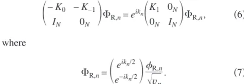
冉
−K0 −K−1IN 0N
冊
⌽R,n=eikn
冉
K1 0N
0N IN
冊
⌽R,n, 共6兲
where
⌽R,n=
冉
eikn/2
e−ikn/2
冊
R,n
冑
vn. 共7兲
Here IN is the N⫻N unit matrix and 0N is the N⫻N zero
matrix 共a general i⫻j zero matrix is denoted as 0i,j兲. The
normalization constant is the square root of the complex group velocityvn=E/kn共ប= 1兲equal to
vn=
i ln
L,n
† 共K
1eikn−e−iknK−1兲R,n, 共8兲
ln=L,n
† 共
S0+S1eikn+S−1e−ikn兲R,n. 共9兲
In the following we assume that the eigenvectors R,n and
L,n are always normalized to give ln= 1. If time-reversal
symmetry holds thenv共knⴱ兲=vnⴱ, so that if the imaginary part
ofknis zero the group velocity is real. Note that, at variance
with Ref. 13, Eq. 共6兲 avoids the inversion of K1, so that it eliminates a possible source of singularities in the calculation of knandR,n.
B. Green’s function
The retarded Green’s functiongzz⬘of the system is defined
by means of the Green’s equation,
兺
z⬘
gzz⬘关共E+i␦兲Sz⬘z⬙−Hz⬘z⬙兴=␦zz⬙, 共10兲
with␦→0+real. In what follows we present and expand, by using left and right Bloch functions, the solution to Eq.共10兲 given in Ref. 13only in terms of the right eigenvectorsR. First we divide the 2NR,nvectors intoNright-going states,
with either Im共kn兲⬎0 共right decaying兲 or Im共kn兲= 0 and vn ⬎0 共right propagating兲, andN left-going states, with either Im共kn兲⬍0 共left decaying兲 or Im共kn兲= 0 and vn⬍0 共left
propagating兲. As a matter of notation in order to distinguish left- from right-going states, in what follows we indicate the right-going states with k,, and vand the left-going states with a bar over these quantities, i.e.,¯k,¯, and¯v.
H
H
1H
0 1
H
[image:2.609.312.558.217.302.2]H
0H
1H
0 0FIG. 1. Schematic representation of the system with onsite HamiltonianH0and hoppingH1. The overlap matrix has the same
As in Ref. 13 we introduce the duals ˜R,n of the
right-going states R,n defined by ˜†R,nR,m=␦nm and the duals
¯˜
R,nof the left-going states¯R,ndefined by¯˜†R,n¯R,m=␦nm. If
we define the matricesQandQ¯ as Q=共R,1 R,2¯R,N兲,
Q ¯ =共¯
R,1 ¯R,2¯¯R,N兲, 共11兲
then the duals can be obtained by simple inversions,
共˜
R,1 ˜R,1¯˜R,N兲=共Q−1兲†,
共¯˜
R,1 ¯˜R,1¯¯˜R,N兲=共Q¯−1兲†. 共12兲
The inversions in Eq.共12兲are usually well defined, unlessQ andQ¯ do not have full rank. We will return on this aspect in Sec. VI, for the moment we assume that the duals can always be constructed.
The Green’s function calculated in Ref.13is then
gzz⬘=
冦
兺
n=1
N
R,ne ikn共z−z⬘兲˜
R,n
† V−1, zⱖz
⬘
兺
n=1
N
¯ R,neik
¯ n共z−z⬘兲¯˜
R,n
†
V−1, zⱕz
⬘
,冧
共13兲
with the matrixV=gzz−1=g00−1given by
V=K−1
冉
兺
n=1
N
e−ikn
R,n˜R,n
† −
兺
n=1
N
e−ik¯n¯
R,n¯˜R,n
†
冊
. 共14兲We now introduce the right transfer matricesTRandT¯R,
TR=
兺
n=1
N
R,neikn˜R,n
†
, 共15兲
T ¯
R=
兺
n=1
N
¯ R,ne−
ik¯n¯˜
R,n
† . 共16兲
These are equivalent to the bulk transfer matrices introduced in Refs.11,12, and24in the context of the recursive Green’s function approach. Note that both TRand¯TR have eigenval-ues with complex modulus ⱕ1. For an integerzthe follow-ing relations hold:
共TR兲z=
兺
n=1
N
R,neiknz˜R,n
† ,
共T¯R兲z=
兺
n=1
N
¯ R,ne−ik
¯ nz¯˜
R,n
†
, 共17兲
which allow us to write the Green’s function of Eq.共13兲as
gzz⬘=
再
共TR兲z−z⬘g
00, zⱖz
⬘
共T¯R兲z⬘−zg00, zⱕz
⬘
.冎
共18兲
In the same way Vis rewritten as
V=g00−1=K−1共TR−1−¯TR兲. 共19兲
Note that although the matricesTRand¯TRare in general well defined, the inverse of these matrices is not. In fact, ifK1and K−1 are singular there are somekn with Im共kn兲→⬁, so that
eikn= 0 共see Sec. IV A兲. In this case T
R does not have full rank and is therefore singular. The same argument holds for T
¯
R. Equation共19兲can therefore be used only if the matrices K1andK−1are not singular.
A possible way for overcoming such limitation is by using an equivalent form for the Green’s function based on the left and right eigenvectors. The starting point is relation 共A6兲 betweenR,nandL,n. This allows us to find the connection
between the duals and the left eigenvectors. Equation 共A6兲 contains a sum over both left- and right-going states. By moving the contribution of the left-going states to the right side of the equation, we obtain兺nN=1R,nL,+n
ivn = −兺n=1 N ¯R,n¯L,+n
i¯vn =B,
where we have introduced the auxiliary matrixB. By multi-plying B from the left with either ˜R† or ¯˜R† we obtain, re-spectively, ˜R,†n=iv1
nL,n
† B−1 and ¯˜ R,n
† = 1 −i¯vn¯L,n
† B−1. The ma-trixBis determined by inserting these relations into Eq.共14兲 and by using identity共A8兲. The result isB=g00. The relation between the dual basis and the left eigenvectors is therefore
˜ R,n
† = 1 ivn
L,†ng00−1, ¯˜R,†n=
1 −iv¯n
¯ L,n
† g 00
−1. 共20兲
This result allows us to rewrite the Green’s function of Eq.
共13兲in a shorter form,
gzz⬘=
冦
兺
n=1
N
1 ivn
R,neikn共z−z⬘兲L,n
†
, zⱖz
⬘
兺
n=1
N
1 −i¯vn
¯ R,neik
¯ n共z−z⬘兲¯
L,n
†
, zⱕz
⬘
.冧
共21兲
This result represents a generalization to complex energies and to systems breaking time-reversal symmetry of the solu-tion given in Refs. 25 and 26 for Hermitian Hamiltonians, real energy, and an orthogonal tight-binding model. This derivation shows that the Green’s function can be equiva-lently expressed by using the right eigenvectors and their duals关Eq. 共13兲兴or both the right and left eigenvectors关Eq.
共21兲兴. It is thus possible to move from one representation to the other through Eq. 共20兲 that relates the duals to the left eigenvectors. One can then decide which representation to use, depending on the specific problem investigated. We note that Eq.共21兲has the benefit thatg00can be calculated also in the case where the two matricesK1andK−1are singular. For those kn where Im共kn兲→⬁ the group velocity becomes vn
=iL,†nK0R,n and is therefore well defined 关¯vn=
−i¯L,n
†
K0¯R,nfor Im共¯kn兲→−⬁兴.
As a matter of completeness we show that a representa-tion entirely based on the left Bloch funcrepresenta-tions and their duals
˜
L,n and¯˜L,n is also possible. By multiplying Eq. 共21兲,
re-spectively, by˜L,nand¯˜L,nfrom the right, we obtain the two
˜ L,n=
1 ivn
g00−1R,n, ¯˜L,n=
1 −i¯vn
g00−1¯R,n. 共22兲
Again the left transfer matricesTL andT¯Lare defined as
TL=
兺
n=1
N
˜
L,neiknL,†n, 共23兲
T ¯
L=
兺
n=1
N
¯ ˜
L,ne−ik ¯
n¯
L,n
†
, 共24兲
and the Green’s function of Eq.共21兲can be rewritten as
gzz⬘=
再
g00共TL兲z−z⬘, zⱖz
⬘
g00共¯TL兲z⬘−z, zⱕz
⬘
.冎
共25兲The structure of Eq.共25兲is the same as that of Eq.共18兲, with the difference that now g00 is multiplied to the left of the transfer matrix. Finally we extend Eq.共19兲and present four equivalent relations for the inverse ofg00,
g00−1=K−1共TR −1
−T¯R兲=K1共T¯R −1
−TR兲
=共TL−1−T¯L兲K−1=共¯TL−1−TL兲K1. 共26兲 The second of these relations can be shown by multiplying Eq.共A7兲byg00−1from the right and then by using Eq.共20兲. In the same way the third and fourth equations can be obtained by multiplying identities共A7兲and共A8兲byg00−1from the left. In the following we will use mostly the quantities expressed in terms of the right eigenvectors only, however the same conclusions can be derived using the left eigenvectors.
C. Density of states
As an example of the use of the Green’s function in the form of Eq. 共21兲, we determine the spectral function A and the density of states 共DOS兲 of the infinite quasi-1D system for the special case where the Hamiltonian and the overlap matrices are Hermitian. The spectral function is defined as1
Azz⬘=i关g−g†兴zz⬘=i关gzz⬘−共gz⬘z兲†兴. 共27兲
The DOSzprojected on the unit cellzthen is
z=
1
2Tr
冋
兺
z⬘ Azz⬘Sz⬘z册
. 共28兲By using Eq.共2兲this becomes
z=
1
2Tr关AzzS0+Az,z−1S1+Az,z+1S−1兴. 共29兲 In general the main contribution originates from the first term in the sum, which can be interpreted as the onsite DOS
˜z,
˜z=
1
2Tr关AzzS0兴. 共30兲 We now calculate A and for the special case where K−1=K1† and K0=K0†. In this case for Im共kn兲= 0 we have
L,n=R,n, whereas if Im共kn兲⫽0 thenL,n=L共kn兲=¯R共knⴱ兲.
In the same way for Im共¯kn兲= 0 we have¯L,n=¯R,n, whereas
if Im共¯kn兲⫽0 then ¯L,n=¯L共¯kn兲=R共¯knⴱ兲. Therefore for each
right-decaying state with Im共kn兲⬎0 there is a left decaying
state with ¯kn=knⴱ and v共¯kn兲ⴱ=v共kn兲. Using these relations
when inserting the Green’s function of Eq. 共21兲in the defi-nition of Azz⬘, the contribution from all the decaying states
cancels out. The only remaining contributions come from the propagating states, also denoted as open channels. For these knⴱ=kn,¯kn= −kn, and v共¯kn兲= −v共kn兲. With these constraints,
and by using Eq. 共21兲, the spectral function becomes
Azz⬘=
兺
n Nopeneikn共z−z⬘兲
vn
R,nR,†n+
e−ikn共z−z⬘兲
vn
¯
R,n¯R,†n, 共31兲
where Nopen is the number of open channels 共number of Bloch functions at a given energy with real positive k vec-tor兲. If there are no open channels Azz⬘= 0 and the Green’s
function is Hermitian. Finally, by using Eqs. 共31兲 and共29兲, and the fact that the eigenvectors are normalized so to give ln= 1关see Eq. 共9兲兴, the DOS at the sitez= 0 is simply
0= 1
兺
n Nopen1
vn
. 共32兲
This is the well-known result for the DOS of infinite periodic 1D systems.27
III. SURFACE GREEN’S FUNCTION AND SELF-ENERGY
The retarded Green’s functiongSfor a quasiperiodic sys-tem, where the left and right sides are separated at the posi-tion z= 0共the left-hand side part extends fromz= −⬁ toz= −1 and the right-hand side part from z= 1 to z=⬁, with no coupling between the cells at z= −1 and z= 1兲, can be con-structed from the Green’s functiongfor the infinite chain as demonstrated in Ref.13,
gS,zz⬘=gzz⬘−gz0g00 −1
g0z⬘. 共33兲
The left-hand side SGF is then defined as GL=gS,−1,−1 and the right SGF as GR=gS,11. The SGF can be obtained by using Eq.共18兲,
GL=共IN−¯TRTR兲g00,
GR=共IN−TRT¯R兲g00. 共34兲 This corresponds to the form derived in Ref.13. This result can be simplified by using relation共26兲for g00 to
GL=T¯RK1−1,
GR=TRK−1 −1
. 共35兲
⌺L=K−1¯TR, 共36兲
⌺R=K1TR. 共37兲
In complete analogy the same expressions obtained by using the left transfer matrices are⌺L=TLK1and⌺R=¯TLK−1. This result is equivalent to those obtained in Refs. 8,11,12, and
14–16and derived with different approaches, demonstrating
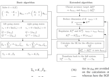
the equivalence of those to our semianalytical formula. Since NEGF-based transport codes simply require⌺L and⌺R, our scheme allows the calculations of system with arbitrarily complicated electronic structure. A schematic tree diagram describing the steps involved in obtaining the SE is shown in Fig.2共basic algorithm兲.
Equations 共36兲 and共37兲 demonstrate that the SE can be calculated directly without explicitly calculatingGLandGR. In situations where also the SGFs are needed, these can be obtained by using the relations
GL= −关K0+⌺L兴−1, 共38兲
GR= −关K0+⌺R兴−1. 共39兲 This can be derived by adding one layer to the left and one to the right surfaces, respectively.9In Appendix B we show that the SEs calculated with Eqs.共36兲and共37兲indeed fulfill the above equation. Moreover with the use of Eqs.共35兲and共38兲 we can now regularize Eq.共19兲also for the case whereTRis singular by writing it as
g00−1= −K0−⌺L−⌺R. 共40兲 We have therefore a scheme where the SEs are identified as the principal quantities, whereas the SGF andg00are derived from these.
When we compare the method of Ref.13with the equa-tions derived above, we notice that now it is not necessary to calculate the matrix g00 and its inverse using Eq. 共19兲 in order to obtain the SE. This is not defined in the case of singular K1 and K−1, and therefore we expect the method presented here to be more stable and accurate. Also the prob-lems caused close to band edges by the Van Hove
singulari-ties ing00are avoided. Moreover the method in Ref.13relies on the calculation of the SGF in order to obtain the SE, whereas here the SGF is not needed. As we will show in Sec. VI close to surface states the error in the SGF is much larger than the one for the SE, so that we also expect a large im-provement in the accuracy for those particular states.
IV. REDUCING THE CONDITION NUMBER OFK1ANDK−1
The accuracy with which the SE is calculated depends on the accuracy involved in solving Eq. 共6兲, a quadratic eigen-value problem extensively studied in the past.22,23 However most solution methods have problems ifK1orK−1 are close to being singular or more generally if their condition number
is large. In this case some of the complex eigenvalues tend to infinity and others to zero at the same time, and this results in a loss of accuracy in numerical computations. When cal-culating TR共¯TR兲 however the contributions from the states with Im共kn兲→⬁ 关Im共¯kn兲→−⬁兴 are vanishingly small. It is
therefore useful to limit the range of the eigenvalues兵eikn其in
such a way that the important eigenstates with small兩Im共kn兲兩
and兩Im共¯kn兲兩can be calculated accurately, while losing
preci-sion for the less important eigenstates with large兩Im共kn兲兩and 兩Im共¯kn兲兩. In this section we show how this can be achieved by
decreasing共K1兲and共K−1兲. Here we assume thatK1=K−1† , so that 共K1兲=共K−1兲. Minor modifications are needed for the general case共see Appendix C兲.
In order to obtain共K1兲first a SVD of the matrix is per-formed,
K1=USV†. 共41兲 Here,UandV are unitary matrices andS is a diagonal ma-trix, whose diagonal elements sn are the singular values.
These are real and positive, and ordered so that sn+1ⱕsn. If
smax is the largest singular value, and smin the smallest one, then the condition number is defined as 共K1兲=smax/smin, withK1 singular ifsminis zero.
We now replace S with an approximate SSVD, whose di-agonal elementssSVD,n are
−K0 −K−1
1 0
ΦR,n=eikn
K1 0
0 1
ΦR,n
TR=
N
i=1 eiknφ
R,nφ˜†R,n
ΣR=K1TR
Σeff
L −→ΣL ΣeffR −→ΣR vn>0∨Im(kn)>0
Q−1†={φ˜R,n}
¯ TR=
N
i=1 e−ik¯nφ¯
R,n˜¯φ †
R,n
¯ Q−1†={φ˜¯
R,n}
¯ Q={φ¯R,n}
Solvek=k(E) Choose accuracy target ∆maxΣ,r
Calculate the SE for the effective system
Basic algorithm
Transform back to the full system.
Extended algorithm
Reduce dimension ofK:sSVD= 0
Σeff
L ΣeffR
δSVD,1
K Keff
left going states right going states
vn<0∨Im(kn)<0
Q={φR,n} RegularizeK
eff
1 andK−eff1: sSVD=smaxδSVD,2 Keff
1 →K1eff,SVD+W(wnoise)
∆eff
Σ,r>∆maxΣ,r ⇒newδSVD,2
∆Σ
,
r
>
∆
ma
x
Σ
,
r
⇒
new
δSV
D
,
1
⇒δSVD,1andδSVD,2≤∆maxΣ,r
[image:5.609.48.401.64.315.2]ΣL=K−1T¯R
sSVD,n=
再
sn, snⱖsmax␦SVD sSVD, sn⬍smax␦SVD
冎
共42兲
and accordinglyK1withK1,SVD=USSVDV†. The tolerance pa-rameter ␦SVD is a real positive number that determines the condition number ofK1,SVD.
We now present two possible choices forsSVD. The first is to set sSVD= 0, resulting in K1,SVD being singular. We can then perform a unitary transformation in order to eliminate the degrees of freedom associated tosSVD,n= 0 and obtain an
effective K1 matrix 共K1 eff兲
with reduced size for which
共K1eff兲ⱕ␦SVD−1 . The second possibility is to set sSVD =smax␦SVD, so that by definition we have 共K1兲=␦SVD−1 . The accuracy obtained with both strategies is similar, the advan-tage of using the first however is that the size of the matrices is reduced, so that for big systems the computation is much faster. In our implementation we use both methods together; first we reduce the size of the system by settingsSVD= 0, and then, if necessary, we further reduce the condition number for the effective system by limiting the smallest singular value.
A. Reduction in system size
Here we set all the M singular values sn smaller than
smax␦SVDto zero, so that there areNeff=N−Msingular values snwithsnⱖsmax␦SVD. The transformations needed in order to obtain the right SE are now presented共the procedure for the left SE is analogous兲. We apply the unitary transformations Kzz
⬘
⬘=U†Kzz⬘U and R,
⬘
n=U†R,n, and we define K1⬘
=U†K1,SVDU, K−1
⬘
=U†K−1,SVDU, and K0⬘
=U†K0U. Since M singular values of K1,SVD are zero the transformed matrices have the structureK1
⬘
=冉
K1,c K1,u 0M,Neff 0M,M冊
, K0
⬘
=冉
A B C D冊
,K−1
⬘
=冉
K−1,c 0Neff,MK−1,u 0M,M
冊
, R,
⬘
n=冉
c,n
u,n
冊
, 共43兲
where the dimensions of the new matrices areNeff⫻Nefffor K1,c,K−1,c, andA,Neff⫻M forK1,uandB,M⫻NeffforK−1,u
andC, andM⫻M forD. Finallyc,nis a column vector of
dimensionNeff, andu,nis of dimensionM. The transformed
form of Eq.共4兲is
共K0
⬘
+K1⬘
eikn+K−1
⬘
e−ikn兲R,n
⬘
= 0. 共44兲Due to the structure of K−1
⬘
there are M solutions to this equation with eikn= 0 andc,n= 0. We therefore split up the
right-going states into those with finite eikn⫽0 and those
witheikn= 0. For the first set, from Eq.共44兲, we obtain
u,n=Fnc,n, 共45兲
with
Fn= −D−1共K−1,ue−ikn+C兲. 共46兲
The c,n are then solutions of an effective system with
re-duced size,
共K0eff+K1effeikn+K
−1 effe−ikn兲
c,n= 0, 共47兲
where the effective matrices are
K1eff=K1,c−K1,uD−1C,
K−1eff=K−1,c−BD−1K−1,u,
K0eff=A−BD−1C−K1,uD−1K−1,u. 共48兲
We can now solve the quadratic eigenvalue problem关Eq.共6兲兴 for this effective system to get the set of Neff eigenvectors Qc=共c,1 c,2¯c,Neff兲and eigenvalues 兵eikn其for the
right-going states. The M eigenvectors of the second set of solu-tions with eikn= 0 are given by
c,n= 0 with a general u,n.
The set of eigenvectors of the full K
⬘
matrix therefore isQ=
冉
Qc 0Neff,MQu Q0
冊
, 共49兲
with Qu=共F1c,1 F2c,2¯FNeffc,Neff兲 and Q0 is a general matrix of solution vectors for the states with eikn= 0. From
this we obtain the set of duals,
Q−1=
冉
Qc−1 0
Neff,M
−Q0−1QuQc
−1
Q0−1
冊
. 共50兲 Using these results we can now calculate the transfer matrix TR⬘
of the transformed system,TR
⬘
=兺
n=1
Neff
eikn
冉
c,n˜
c,n
† 0N
eff,M
Fnc,n˜c,n
† 0
M,M
冊
, 共51兲
where we have also used the fact thateikn= 0 for the second
set of solutions. We note that setting theM smallest singular valuessnto zero causes the lastMcolumns ofTR
⬘
to be zero too. Moreover the explicit calculation ofQ0is not needed in order to obtainTR⬘
. From this and Eq.共37兲we obtain the right SE,⌺R
⬘
=冉
⌺Reff−K1,uD−1K−1,u 0Neff,M
0M,Neff 0M,M
冊
, 共52兲
where
⌺Reff=K1eff
兺
n=1
Neff
eikn
c,n˜c†,n 共53兲
is the SE of the effective system.
The structure of ⌺R
⬘
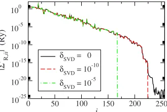
shows that by applying this unitary transformation, we have ordered the elements of the SE by absolute size, moving those columns共rows兲with the smallest values to the right共bottom兲. By setting the smallest singular values ofK1to zero, those columns and rows of the SE with small values have also been set to zero. This is illustrated in Fig.3, where the absolute value of the diagonal elements of the transformed self-energy兩⌺R,⬘
ii兩is shown for a共8,0兲zigzagcarbon nanotube at the Fermi energy EF 共see Sec. V for a detailed description of the system兲. The 兩⌺R,
⬘
ii兩 are basicallyin-creasing value of␦SVDresults in more diagonal elements of
⌺R
⬘
set to zero. We note thatNeffis of similar size asNin Fig. 3, since the system is rather short alongzand a small basis set is used共i.e.,Nis small兲. For large systems and rich basis sets the ratio Neff/N will decrease. The physical interpreta-tion of the zero columns and rows in the SE is that the M states withkn→⬁decay infinitely fast, so that the interactionof those states is limited to the site they are localized at. Finally the SE of the original system can be obtained by applying the inverse unitary transformation,
⌺R=U⌺R
⬘
U†, 共54兲and in contrast to⌺R
⬘
the matrix⌺Ris a denseN⫻Nmatrix. Note that in order to obtain the left SE we perform the unitary transformations Kzz⬘
⬘=V†Kzz⬘V and R,⬘
n=VR,n andthen follow an analogous procedure. In this case however instead of the right-going states the left-going ones are used.
B. Limiting the smallest singular value
We can limit the lower bound of the singular valuessnby
settingsSVD=smax␦SVDin Eq. 共42兲. In this case the approxi-matedKmatrix is obtained by replacingK1withK1,SVD. The error introduced is now of the order of smax␦SVD. Ideally smax␦SVD should be of the order of the machine numerical precision, so that the error is minimal. However sometimes increasingsmax␦SVD beyond that value improves the results, therefore␦SVDis left as a parameter to adjust depending on the material system investigated. This will be discussed ex-tensively in Sec. V.
A simpler but equally effective possibility for limiting the smallest singular value of a matrix is that of adding a small random perturbation.17,28Thus another strategy for reducing the condition number of K1 is that of replacing K1 with K1,noise=K1+W共wnoise兲, where W共wnoise兲 is a matrix whose elements are random complex numbers with an average ab-solute value兩Wij兩⬃wnoise. In particular we choose the兩Wij兩in
such a way that both Re共Wij兲 and Im共Wij兲are random
num-bers in the range 关−wnoise,wnoise兴. We find that if wnoise =smax␦SVD the addition of noise usually gives results as ac-curate as those obtained with the SVD procedure, but the calculation is faster since instead of performing a SVD we just perform a sum of the matrices.
In Fig.2we present our final extended algorithm as it has been implemented in SMEAGOL. This now includes the
fol-lowing regularization procedure of K1. First the size of K1 and hence of the whole problem is reduced by using the scheme described in Sec. IV A, with a tolerance parameter
␦SVD=␦SVD,1. This generates an effective matrixK1effwhose condition number共K1eff兲is reduced by adding a small noise matrixW共wnoise兲. Such a step is extremely fast and enhances considerably the numerical stability of the calculation. In most cases the SE for the effective system can then be cal-culated and no further regularization steps are needed. How-ever, in some cases the calculation of the SE still fails. This, for example, happens when the solution of Eq. 共6兲 for the effective system fails or else when the calculated number of left-going states erroneously differs from the number of right-going states. In these critical situations we further de-crease 共K1eff兲by limiting the smallest singular value ofK1eff as described in Sec. IV B with a tolerance parameter ␦SVD =␦SVD,2. The code automatically adjusts ␦SVD,1, ␦SVD,2, and wnoisewithin a given range until the SE is calculated. In our test calculations for a number of different systems we found no situation where such a scheme has failed. In contrast when the standard algorithm of Ref. 13 is employed the number of failures was considerable. Note that our extended algorithm can also be used in conjunction with recursive methods for evaluating the SE.9–12Also in this case it will decrease the computing time for large systems due to the reduced size of the effective Kmatrix.
V. ERROR ANALYSIS
When recursive algorithms are used the accuracy of the SE is automatically known as it coincides with the conver-gence criterion. Poor converconver-gence is found when the error cannot be reduced below a given tolerance. Direct methods, as the one presented here, are in principle error free in the sense that when the solution is found, this is in principle exact. For this reason the numerical errors arising from direct schemes usually are not estimated. In this section we per-form this estimate and present a detailed error analysis for three different material systems.
In order to estimate the numerical accuracy we use the recursive relations of Eqs.共38兲and共39兲, written as
⌺L out
= −K−1关K0+⌺L in兴−1K
1,
⌺Rout= −K1关K0+⌺Rin兴−1K−1, 共55兲 where⌺兵inL/R其are calculated with our extended algorithm and
⌺兵outL/R其 are obtained by evaluating the right-hand side term of
the above equations. When the solution is exact then ⌺Lout =⌺Linand⌺Rout=⌺Rin. Therefore we can define a measure of the error⌬⌺as
⌬⌺=储⌺兵L/R其 out
−⌺兵inL/R其储max, 共56兲 where 储¯储max stands for the maximum norm,18 the corre-sponding relative error is⌬⌺,r=⌬⌺/储⌺兵L/R其储max. The accuracy criterion used in the extended algorithm is the following. We first set ␦SVD,1, wnoise, and eventually ␦SVD,2 and compute
⌬⌺,r. This should be lower than a target accuracy⌬⌺,r max. If this is not the case then the SE will be recalculated with a
differ-0 50 100 150 200 250
i 10-25
10-20 10-15 10-10 10-5 100
|
Σ
’R,ii
|
(Ry
)
δSVD= 0
δSVD= 10-10
[image:7.609.91.256.68.179.2]δSVD= 10-5
ent set of tolerance parameters, until⌬⌺,rreaches the desired accuracy. If this condition is never achieved the final SE is the one with the smallest⌬⌺,r.
We now calculate the SE for different variations of the method, chosen in order to highlight the problems arising from K1 and K−1 and to show the difference between the basic method of Ref. 13and the extensions presented here. There are two main differences between the two methods. The first is that here we solve Eq.共6兲without invertingK1, whereas in Ref. 13 K1−1 is used to solve the inverse band-structure relation k=k共E兲. Clearly this second choice is less accurate ifK1is close to singular. However it is much faster computationally, so that it might be of advantage for big systems. The second difference is that here it is not necessary to calculate g00 via Eq. 共19兲, so that one does not need to invertTRand¯TR.
In order to investigate the effect of these two aspects in-dependently, we have calculated the SE using the following four methods. In method 1 we use the algorithm presented in this work. In particular we use Eq.共6兲to solve the quadratic eigenvalue problem and Eqs.共36兲and共37兲to obtain the SE
共for the right SE we actually use a different form of Eq.共6兲; see Appendix D兲. Method 2 is essentially the same, with the only difference that instead of solving Eq. 共6兲 we use the eigenvalue method of Ref.13. In method 3 we solve Eq.共6兲, but we use Eq. 共34兲to calculate the SGF, withg00 obtained from Eq.共19兲. Finally method 4 is the algorithm of Ref.13. In order to obtain a statistically significant average of the errors, we plot a histogram of the calculated errors for both
⌺Land⌺Rfor a large energy range. Here we use the absolute error, since it can readily be compared to the energy scale of the problem. Note that although the relative error might be small, the absolute error can be very large if 储⌺兵L/R其储max
Ⰷ1 Ry. Furthermore in order to keep the analysis simple in all the calculations of this section, we do not reduce the system size nor do we add noise 共wnoise= 0兲. We regularize K1 andK−1 by using sSVD=smax␦SVD in Eq. 共42兲. Since the error depends on the chosen␦SVD, here we calculate⌬⌺for a set of␦SVD in the range共0 , 10−23, 10−22, . . . , 10−4, 10−3兲. We then present the smallest ⌬⌺ found for ␦SVD taken in that range. This is the smallest possible error achievable with a given method and allows us to extract information on the range of optimal SVD values for a given method.
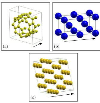
As first example a共8,0兲zigzag carbon nanotube29is pre-sented关the unit cell is shown in Fig.4共a兲兴. The length of the periodic unit cell is 4.26 Å along the nanotube, with 32 car-bon atoms in the unit cell. The LDA approximation共no spin polarization兲 is used for the exchange-correlation potential. We consider 2sand 2p orbitals for carbon with doubleand a cutoff radius rc for the first of rc= 5 bohr. Higher are
constructed with the split-norm scheme with a split norm of 15%.21 The real-space mesh cutoff is 200 Ry. The matrices
H0, H1, S0, and S1 are extracted from a ground-state DFT calculation for an infinite periodic nanotube. We calculate the SE for the semi-infinite nanotube at 1024 energy points in a range of⫾5 eV around the Fermi energy.
Figure 5共a兲shows the histogram of the errors in the SE, whereNis the number of times a given error⌬⌺appears. In general the figure shows that for this system the average
error increases when going from method 1 to method 2 and method 3, and finally to method 4. The error obtained with method 1 is on average about 6 orders of magnitude smaller than the one obtained with method 4. The main reason be-hind this dramatically improved accuracy is that method 1 does not involve any steps where a singular K1 leads to di-vergencies. Method 4 on the other hand is strongly depen-dent on the condition number ofK1, since it necessitates to invert K1 andTR 共or¯TR兲. Methods 2 and 3 are on average about 1 order of magnitude more precise than method 4. Since they both still involve one of the two inversions, the difference is however not large.
Figure 6共a兲 shows the histogram of the optimum ␦SVD used for the calculations of the SE. Here we plot the number of times N a particular␦SVDhas given the smallest error in the set of calculations. A larger optimal value for ␦SVD indi-cates a stronger dependence of the computational scheme on
共K1兲. For method 1 the range of used ␦SVDis smaller than 10−12. If we force ␦
SVD to be zero we get almost the same level of accuracy, as shown in Fig.5共a兲, which confirms that
(a) (b)
[image:8.609.351.518.66.239.2](c)
FIG. 4. 共Color online兲 Unit cells of the three systems investi-gated in this work: 共a兲 共8,0兲 zigzag carbon nanotube, 共b兲 bcc Fe oriented along the共100兲direction, and共c兲fcc Au oriented along the 共111兲direction. The black arrow indicates the direction of the stack-ingz, i.e., the direction of the transport.
1 102 104
N
1 102 104
N
10-15 10-12 10-9 10-6 10-3 100 103
∆Σ(Ry) 1
102 104
N
method 1 method 2 method 3 method 4
(a)
(b)
(c)
[image:8.609.350.517.557.692.2]the accuracy for method 1 depends little on 共K1兲 for this system. However also for this method there is a set of ener-gies共a few percent of the total number兲where the solution of Eq. 共6兲fails if ␦SVDis too small. The optimal ␦SVD for the other methods is orders of magnitude larger than that of method 1, and it is never smaller than 10−9. The absolute error induced by replacing K1 by K1,SVD is of the order of
␦SVDsmax. Usually smax is of the order of 1 Ry, so that the error is of the order of ␦SVDRy. Therefore since in methods 2–4 a large value of ␦SVD is needed in order to improve
共K1,SVD兲, also the resulting error is large.
The second example is bcc Fe关Fig.4共b兲兴, oriented along the 共100兲 direction. The lattice parameters are the same as in Ref. 30. There are four Fe atoms in the unit cell. We apply periodic boundary conditions in the direction per-pendicular to the stacking, so that these correspond to four Fe planes. The length of the cell along the stacking direction is 5.732 Å. Double- s共rc= 5.6 bohr兲, single-
p共rc= 5.6 bohr兲, and single-d共rc= 5.2 bohr兲bases are used.
The real-space mesh cutoff is 600 Ry, and the DFT calcula-tion is converged for 7⫻7 k-points in the Brillouin-zone orthogonal to the stacking. The SEs have been calculated for the converged DFT calculation at 32 different energies in a range of ⫾1 eV around the Fermi energy and for 10 000 k-points in the two-dimensional共2D兲Brillouin zone perpen-dicular to the stacking direction. For eachk-point there is a different set of matrices K0, K1, and K−1, so that for each k-point there is a different SE. The histogram for the error of the calculated self-energy ⌬⌺ is shown in Fig. 5共b兲 and the histogram for the optimal ␦SVD in Fig. 6共b兲. The general behavior is similar to the one found for the carbon nanotube. We note that, although for the vast majority of the calcula-tions the error in the SE is small, there is a long tail in the histograms of Fig. 5共b兲 indicating the presence of a small number of large errors. This is present for all the methods, with maximum errors of 10−2 Ry for method 1 and 100 Ry for method 4. Closer inspection shows that the reason for the increase in the error for certain energies and k-points is caused by a divergence in储⌺兵L,R其储max. This will be illustrated in more detail in Sec. VI.
Finally we consider fcc Au 关Fig.4共c兲兴, with the stacking along the 共111兲 direction. The unit cell consists of three
planes of nine gold atoms each. These are the typical leads used for the calculations of the transmission properties of molecules attached to gold.31–34 We use double s共r
c
= 6.0 bohr兲and singled共rc= 5.5 bohr兲and fourk-points in
the Brillouin zone perpendicular to the stacking. The mesh cutoff is 400 Ry. The SEs have been calculated for 418 en-ergy points from about 15 eV below to about 10 eV above the Fermi energy. The general behavior关Figs.5共c兲and6共c兲兴 is again similar to that of the previous examples. Also here the error for method 1 is about 6 orders of magnitude smaller than that of method 4, with methods 2 and 3 giving some marginal improvement.
Our results show that the scheme presented here in gen-eral allows the calculation of the SE with high accuracy. The main advantage of method 1 is rooted in the possibility of using a much smaller␦SVD. For big systems sometimes one might prefer to use method 2, since it is considerably faster than method 1 and gives the second best accuracy. In this case we first calculate the SE with method 2 and check the error. Only for those energy points where the error is above some maximum value 共of the order of 10−5 Ry, for ex-ample兲, the calculation is repeated with method 1 to improve the accuracy. Finally the results show that for all methods the SVD transformation ofK1is necessary, although for method 1 it is needed only a few percent of the times. For big sys-tems, in particular if the unit cell is elongated along the stacking direction, or if a rich basis set is used, 共K1兲 will generally increase as there will be some singular values ofK1 going to zero. In these cases also method 1 will require a SVD transformation for most energies. The range of ␦SVD should however be similar to the one shown in Fig.6, so that also the error in the SE should be of the same order of mag-nitude. We also note that in order to keep the analysis sim-pler, here we have not used the reduction in system size described in Sec. IV A, for such large systems it is however crucial in order to decrease the computational effort and regularizeK1 at the same time.
VI. SURFACE STATES
The center of the error distribution for method 1共Fig.5兲 is located at small⌬⌺, usually smaller than 10−11 Ry. How-ever the histogram has also a tail reaching up to very large errors. These are found only at some critical energies as dem-onstrated in Fig. 7共a兲, where we show ⌬⌺ for the carbon nanotube calculated over 1024 energy points in a range of 2 eV around the Fermi energy. The average error is of the order of 10−12 Ry, but at energies around −0.8 and −0.34 eV the error drastically increases. Indeed a finer energy mesh at these points suggests a divergence. The origin of the large errors at particular energies can be investigated by looking at the eigenvalues gL,i of the SGF GL. In Fig. 7共b兲the largest and the smallest absolute values for the eigenvalues, respec-tively, gL,max andgL,min, are plotted as a function of energy
共gL,minⱕ兩gL,i兩ⱕgL,max兲. It can be seen that gL,max diverges close to the energies where the error increases, i.e., we can associate large errors in GL with a divergence in its spec-trum. Since⌺L is calculated from Eq.共36兲the only possible origin for the divergence is in the norm of some of the¯˜R,n.
1 102 104
N
1 102 104
N
0 10-20 10-16 10-12 10-8 10-4 100 δSVD
1 102 104
N
method 1 method 2 method 3 method 4
[image:9.609.89.256.68.209.2](a) (b) (c)
FIG. 6. 共Color online兲 Histogram of␦SVD giving the smallest
error in the self-energy:共a兲 共8,0兲 zigzag carbon nanotube,共b兲 bcc Fe, and共c兲fcc Au.Nis the number of times a given␦SVDgenerates
As these are obtained by inverting the matrix Q¯ =共¯R,1 ¯R,2¯¯R,N兲 关Eq. 共11兲兴, one deduces that the set of
vectors兵¯R,n其is not linearly independent. For these energies
共Q¯兲→⬁. We therefore can simply check the magnitude of
共Q¯兲 to determine whether there is a divergence of the SE close to a particular energy.
Physically the divergence of the SE translates into the presence of a surface state at that particular energy.9,11 Con-sider the spectral representation ofGL,
GL共E兲=
兺
n=1
N
1 E+i␦−En
n˜n
†
, 共57兲
whereEnare the eigenvalues,nare the right eigenvectors of
the effective surface Hamiltonian matrix H0−⌺L with over-lap S0, and ˜n are the left eigenvectors of the same
Hamil-tonian. A localized surface state is found when there is a real eigenvalue En共E兲 at En共E兲=E 共or more generally if
Im关En共E兲兴is very small兲.
From the recursive relation关Eq.共38兲兴one can deduce that for an infinite eigenvalue there is also a corresponding van-ishing eigenvalue. Therefore in Fig. 7共b兲for energies where gL,max→⬁ we have alsogL,min→0. Close to the singularity we can therefore expand the two eigenvalues as gL,max
⬀ 1
E+i␦−En andgL,min⬀E+i␦−En. ForE=Enthe largest
eigen-value in Eq. 共57兲 is then equal to ␦−1, and the smallest is equal to ␦. To avoid divergence therefore the magnitude of the GL eigenvalues can be bounded to a finite value ␦−1by introducing a small imaginary part to the energy for energies in the vicinity of a surface state.
Another possibility for limiting the size of gL,max is to bound the singular values ofQ¯ from below in the same way as it is done forK1共Sec. IV B兲. This essentially imposes the
¯
R,n to be linearly independent from each other. However,
with this scheme it is not possible to conserve the Green’s function causality, so that the SGF might have eigenvalues lying on the positive imaginary axis. Moreover we loose control over the accuracy of the computed SGF and SE. Both these problems are avoided when using a finite␦.
We now investigate the DOS and transport properties of a system when the finite imaginary part ␦ 共broadening兲 is added to the energy. We consider as an example the carbon nanotube of Fig.4. In Fig.8共a兲the onsite surface DOS˜0as defined in Eq. 共30兲 is shown for ␦= 0 Ry, ␦= 10−6 Ry, ␦ = 10−5 Ry, and␦= 10−4 Ry. For␦= 0 the surface DOS van-ishes for energies between −0.42 and +0.39 eV, indicating the presence of a gap around the Fermi energy. Note that there are no Van Hove singularities in ˜0, since we never divide by the group velocity when calculating the SGF. For finite ␦ and energies away from the band gap, the DOS is essentially identical to that calculated for ␦= 0, however in-side the gap˜0does not vanish but saturates to a small value proportional to ␦−1. Moreover whereas the surface states are not visible for␦= 0, they appear in the DOS for finite␦, and their full width at half maximum共FWHM兲equals 2␦.
We then move to the transport by calculating the trans-mission coefficient2T共E兲for a carbon nanotube attached to semi-infinite leads made from an identical carbon nanotube. Since this is a periodic system T共E兲must equal the number of open channels, so that it can only have integer values. This is indeed the case for␦= 0关Fig.8共b兲兴. For finite␦sthe transmission coefficient is only approximately an integer, es-pecially inside the energy-gap region where the finite surface DOS introduced by ␦ leads to a nonzero transmission. The transmission in the gap is proportional to ␦2 共note that the scale is logarithmic兲, since on both sides of the scattering region the artificial surface DOS is proportional to␦. In this region of small transmission therefore the results might change by orders of magnitude depending on the value of␦. For all values of ␦ however we find no contributions to the transmission coming from the surface state, indicating that these do not carry current. These results show that adding a finite value ␦ to the energy has little effect on the actual transmission if this is large. However when the transmission is small, as in the case of tunnel junctions, the finite␦ intro-duces an additional contribution to the conduction that might arbitrarily affect the results. It is thus imperative for those systems to identify surface states and use the imaginary ␦ only in a narrow energy interval around them.
Finally we can give an estimate of the relative accuracy
⌬⌺,r共␦兲=⌬⌺/储⌺储max at the energy corresponding to the
sur-10-12
10-10
10-8
∆Σ
(Ry)
-1 -0.5 0 0.5 1
E-EF(eV)
10-3
100
103
gL
(Ry
-1 )
gL,max
gL,min
(a)
[image:10.609.353.518.68.184.2](b)
FIG. 7. 共Color online兲The error analysis for the carbon nano-tube of Fig.4:共a兲absolute error⌬⌺of the self-energy as a function of the energyE;共b兲 maximum共gL,max兲 and minimum 共gL,min兲
ei-genvalues ofGL.
10-3 100 103
ρ0
(arb.
units) 100-0.34 -0.338 -0.336
103 106
-1 -0.5 0 0.5 1
E-EF(eV)
10-9 10-6 10-3 100
T
δ= 0 δ= 10-6Ry δ= 10-5Ry δ= 10-4Ry (a)
(b)
~
[image:10.609.88.256.69.190.2]face state. As discussed before the origin of the error is the inversion of Q¯ needed to calculate the duals. The relative error introduced by the inversion of Q¯ is proportional to
共Q¯兲.17,18,28,35,36Close to a surface state the smallest singular value is of the order of ␦, so that共Q¯兲⬀␦−1. As this is the dominant source of error in the calculation of the SE close to a surface state, we can approximate the relative error as
⌬⌺,r in
=c1␦−1, 共58兲
wherec1is a constant that depends on the machine precision and on the details of the algorithm. The label “in” explicitly indicates that this is the error in the SE calculated with the extended algorithm 关⌺兵inL/R其 in Eq. 共55兲兴. The absolute error
⌬⌺inis equal to the relative error times储⌺储
max, which is itself proportional to␦−1, so that we get⌬
⌺
in⬀␦−2.
When using Eq. 共56兲 to estimate the error in the SE we introduce an additional error due to the inversion involved in obtaining GL. The largest singular value of GL is propor-tional to␦−1, and the smallest one is proportional to␦, so that the relative error introduced by the inversion is proportional to 共GL−1兲=共GL兲⬀␦−2. For small ␦ we can therefore write for the error in ⌺Lout,
⌬⌺,r out
=c2␦−2, 共59兲
wherec2is again a constant. Since the errors are random the total estimated error can be approximated by adding the con-tributions from the two inversions,
⌬⌺,r 2 ⬇ 共⌬
⌺,r in 兲2+共⌬
⌺,r
out兲2. 共60兲
⌬⌺,ris therefore a good estimate for the true error⌬⌺,r in
if⌬⌺out,r is small. Close to surface states however⌬⌺out,rⰇ⌬⌺in,r, so that
⌬⌺,rlargely overestimates the true error.
To verify these estimates numerically we present a scheme for calculating⌬⌺in,rand⌬⌺out,rindependently. For each SE we perform a second calculation where we add a small amount of noise to the input matricesK0,K1, andK−1, so that we obtain the self-energy ⌺L,noisefor a slightly turbed system. The noise is added as a random relative per-turbation of each element of the matrices. As we decrease the magnitude of the noise the difference between⌺Land⌺L,noise is reduced until it becomes constant for noise smaller than a critical value. In this range of minimum noise even if the difference in the input matrices decreases, the difference in the output matrices is constant, it therefore corresponds to the error in the calculation. As one might expect we find that this critical value of noise is of the same order of mag-nitude as the numerical accuracy used共approximately 10−15 in our calculations兲. We can therefore obtain ⌬⌺in,r=储⌺Lin −⌺L,noisein 储max/储⌺L
in储
max and ⌬⌺,r out
=储⌺Lout−⌺L,noiseout 储max/储⌺L out储
max, with the magnitude of the noise equal to the critical value.
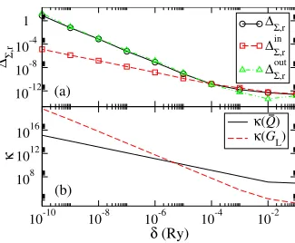
We have calculated the maximum error for a set of 128 energy points located within 10−11 Ry around the energy of the surface state at −0.34 eV for different values of␦. The result is shown in Fig.9共a兲. Indeed for small ␦ ⌬⌺in,r follows Eq. 共58兲 withc1⬇10−15 Ry, ⌬
⌺,r
out follows Eq. 共59兲 with c 2
⬇10−19 Ry2, and 共⌬⌺,r兲2⬇共⌬⌺,r in 兲2+共⌬
⌺,r
out兲2. In Fig. 9共b兲 the condition numbers 共Q¯兲 and 共GL兲 are shown, confirming
共Q¯兲⬀␦−1 and共G
L兲⬀␦−2. This demonstrates that close to surface states⌬⌺,ris mainly caused by the calculation ofGL. Thus ⌬⌺,r largely overestimates the real error ⌬⌺,r
in
, which even for␦= 10−10 Ry has an acceptable size of⌬
⌺,r in ⬇10−5. Since c1 andc2 are generally system dependent, in prac-tical calculations we use a value of ␦ ranging between 10−7 and 10−6 Ry for energies in the vicinity of surface states, mainly in order to limit the absolute error. Moreover ␦ is added in an energy range corresponding approximately to the FWHM of the imaginary part of 共E−En+i␦兲−1, which is
equal to 2␦. Although this range is only of the order of 10−7− 10−6 Ry, in practical calculations where both energy andk-point sampling are fine, the number of times when this prescription is applied can be rather large共see Fig.5兲.
The above analysis confirms that close to surface states also direct methods have the same accuracy problems of re-cursive methods. This fact is usually ignored in the literature,4,13,14,30 where it is assumed that the accuracy is constant for a given algorithm. Here we show that the accu-racy of a method is solely determined by the value of c1, which, as indicated in Sec. V, can vary over many orders of magnitude. Our analysis also shows that methods requiring the explicit calculation ofGL from its inverse are much less accurate close to surface states than those calculating ⌺L directly.
VII. CONCLUSIONS
By extending the scheme proposed in Ref. 13, we have presented a different but equivalent form for calculating the Green’s functions of an infinite quasi-1D system, as well as the SGF and SE for the semi-infinite system. We have then constructed an extended algorithm containing also the neces-sary steps to regularize the ill conditioned hopping matrices. This is found to be crucial in order to obtain a numerically stable algorithm. By applying a unitary transformation based on a SVD, we remove the rapidly decaying states and calcu-late the SE for an effective system with reduced size. We further decrease the condition number of the hopping matri-ces by adding a small random perturbation and by limiting the smallest singular value.
10-12
10-8
10-4
1
∆Σ,r
∆Σ,r ∆Σin,r ∆Σout,r
10-10 10-8 10-6 10-4 10-2
δ(Ry)
108
1012
1016
κ
κ(Q) κ(GL)
[image:11.609.355.518.66.200.2](b) (a)
FIG. 9. 共Color online兲 共a兲Relative error of the self-energy⌬⌺,r
共⌬⌺,r
in represents the true error兲, 共b兲 condition number of Q¯ and GL, as a function of the broadening␦ for the carbon nanotube of
We have performed a detailed error analysis on the nu-merical calculation of the SE, showing that if the algorithm does not involve an inversion of the hopping matricesK1共or K−1兲high accuracy is obtained. We also find that the error is not constant as a function of energy. It is shown that an increase in accuracy is needed especially close to energies where the SE and SGF diverge, which corresponds to the presence of surface states in the semi-infinite system. At these energies we improved the accuracy by adding a small imaginary part to the energy. We have shown that this pro-cedure affects the transport properties little in the high trans-mission limit. However, for low transtrans-mission this adds some spurious surface density of states contributing significantly to the total transmission. The transport can therefore be strongly affected, so that the imaginary part should be added only in a small energy range around the poles and it should be as