Surface scanning with uncoded structured light sources

(1)

ROBINSON, Alan.

Available from Sheffield Hallam University Research Archive (SHURA) at:

http://shura.shu.ac.uk/20284/

This document is the author deposited version. You are advised to consult the

publisher's version if you wish to cite from it.

Published version

ROBINSON, Alan. (2005). Surface scanning with uncoded structured light sources.

Doctoral, Sheffield Hallam University (United Kingdom)..

Copyright and re-use policy

(2)

(3)

INFORMATION TO ALL USERS

The qu ality of this repro d u ctio n is d e p e n d e n t upon the q u ality of the copy subm itted.

In the unlikely e v e n t that the a u th o r did not send a c o m p le te m anuscript and there are missing pages, these will be note d . Also, if m aterial had to be rem oved,

a n o te will in d ica te the deletion.

uest

ProQuest 10700929

Published by ProQuest LLC(2017). C op yrig ht of the Dissertation is held by the Author.

This work is protected against unauthorized copying under Title 17, United States C o d e M icroform Edition © ProQuest LLC.

ProQuest LLC.

789 East Eisenhower Parkway P.O. Box 1346

(4)

Alan Robinson

A thesis submitted in partial fulfilment o f the requirements of

Sheffield Hallam University

for the degree of Doctor of Philosophy

(5)

Abstract

Structured Light Scanners measure the surface of a target object, producing a set of vertices

which can be used to construct a three-dimensional model of the surface. The techniques are

particularly appropriate for measuring the smoothly undulating, featureless forms which Stereo

Vision methods find difficult, and the structured light pattern explicitly gives a dense graph of

connected vertices, thus obviating the need for vertex- triangulation prior to surface

reconstruction. In addition, the technique provides the measurements almost instantaneously,

and so is suitable for scanning moving and non-rigid objects. Because of these advantages there

is an imperative to extend the range of scannable surfaces to those including occlusions, which

often reduce or prevent successful measurement.

This thesis investigates ways of improving both the accuracy and the range of surface

types which can be scanned using structured light techniques, extending current research by

examining the role of occlusions and geometric constraints, and introducing novel algorithms to

solve the Indexing Problem. The Indexing Problem demands that for every pattern element in

the projected image, its counterpart, reflected from the surface of the target object, must be

found in the recorded image, and most researchers have declared this problem to be intractable

without resorting to coding schemes which uniquely identify each pattern element. The use of

urtcoded projection patterns, where the pattern elements are projected without any unique

identification, has two advantages: firstly it provides the densest possible set of measured

vertices within a single video timeframe, and secondly it allows the investigation of the

fundamental problems without the distraction of dealing with coding schemes. These

advantages educe the general strategy adopted in this thesis, of attempting to solve the Indexing

Problem using uncoded patterns, and then adding some coding where difficulties still remain.

In order to carry out these investigations it is necessary to precisely measure the system

and its outputs, and to achieve this requirement two scanners have been built, a Single Stripe

Scanner and a Multiple Stripe Scanner. The Single Stripe Scanner introduces the geometric

measurement methods and provides a reference output which matches the industry standard; the

Multiple Stripe Scanner then tests the results of the investigations and evaluates the success of

the new algorithms and constraints. In addition, some of the investigations are tested

(6)

Indexing Problem can often be completely solved if the new indexing algorithms and geometric

constraints are included. Furthermore, while there are some cases where the Indexing Problem

cannot be solved without recourse to a coding scheme, the addition of occlusion detection in the

algorithms greatly improves the indexing accuracy and therefore the successful measurement of

(7)

Publications

A. Robinson, L. Alboul and M.A. Rodrigues, Methods fo r Indexing Stripes in Uncoded

Structured Light Scanning Systems, Journal of WSCG, 12(3), pp. 371-378, 2004.

M.A. Rodrigues and Alan Robinson, Image Processing Method and Apparatus, Rotational

Position Estimator and 3D Model Builder (Tripods), UK Patent Application 0402420.4,

February 4th, 2004.

M.A. Rodrigues, Alan Robinson and Lyuba Alboul, Apparatus and Methods fo r Three

Dimensional Scanning, Multiple Stripe Scanning Method, UK Patent Application No.

(8)

Acknowledgments

The author would like to thank the Geometric Modelling and Pattern Recognition group of

Marcos Rodrigues,

Lyuba Alboul,

Georgios Chliveros,

Jacques Penders,

Gilberto Echevarria,

David Cooper,

Charilaos Alexakis and

Alexander Chamski,

at Sheffield Hallam University for their unstinting help in producing this thesis. Many thanks

must also go to Sanaz Jabbari for help in formulating the system geometry.

(9)

List of Figures

Figure 1.3.1: The structured light scanning system...4

Figure 1.3.2: Stripe coding schemes...5

Figure 1.6.1: Visualisation of the stripe pattern...8

Figure 1.6.2: Recorded image from structured light scanner (part)... 8

Figure 1.7.1: Synthetic pattern of stripes showing two possible interpretations...9

Figure 1.9.1: Horizontal step (left), and lateral translation (right)... 11

Figure 3.7.1: Steps in the Investigation Process... 31

Figure 4.1.1: The Single Stripe Scanner... 33

Figure 4.1.2a: The apparatus viewed "from above"... 34

Figure 4.1.2b: The apparatus viewed "from the side"... 35

Figure 4.1.3: Transformation of the image into the system space...36

Figure 4.3.1: Luminance across one row in the pixel array... 38

Figure 4.3.2a: Laser stripe projected onto folded paper...39

Figure 4.3.2b. Depth profile from Figure 4.3.2a...39

Figure 4.3.3: Possible values of 8i constrained to 4 decimal places... 40

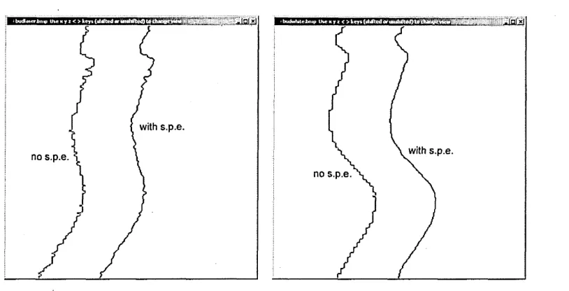
Figure 4.4.2: Profile of scanned ramp with and without subpixel estimation... 44

Figure 4.4.3.Detail of scanned terracotta head, using laser light (left) and white light (right)... 45

Figure 4.4.4: Depth profiles of Figure 4.4.3... 46

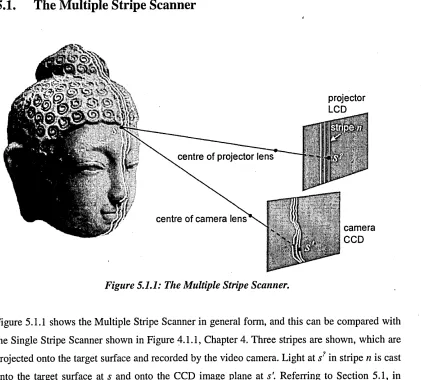
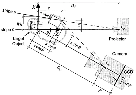
Figure 5.1.1: The Multiple Stripe Scanner...48

Figure 5.2.1a: The Multiple Stripe Scanner viewed "from above"... 50

Figure 5.2.1b: The Mulitple Stripe Scanner viewed "from the side"... 50

Figure 5.3.1: Condition where the target surface is infinitely far away...54

Figure 5.5.1: The six data structures...56

Figure 5.6.1: Calibration chart showing lens distortion...61

Figure 5.6.4: The projector calibration image...63

Figure 5.6.5: Calibration chart viewed in bitmap image...64

Figure 6.2.1: Detail from recorded image showing disconnected stripe...69

Figure 6.3.1: Epipolar geometry for stereo vision system... 70

Figure 6.3.2: Rectification of stereo images... 71

Figure 6.4.1: Epipolar geometry for a Structured Light System... 72

(16)

Figure 6.6.1: Finding epipolar lines corresponding to specific dots... 76

Figure 6.7.1: Theoretical positions of epipolar lines for specific dots...78

Figure 6.9.1: Rectification by spatial positioning...81

Figure 6.10.1: Projection of vertical stripe...83

Figure 6.10.2: Stripes "broken" by occlusion... 84

Figure 6.11.2: Dot and stripe projections... 84

Figure 7.2.1: Processing the recorded image... 88

Figure 7.5.1: Moving around the peaks data...91

Figure 7.9.1: Illustration of patches, boundaries and neighbourhoods... 94

Figure 7.10.1: Indexing using Scanline methods...96

Figure 7.12.1: Indexing using Scan and Search methods... 98

Figure 7.15.1: The Flood Filler... 102

Figure 7.18.1: Northern and southern disconnections... 104

Figure 7.18.2: Indexing with the Scanline method (left), the Scan and Search method (centre) and the Flood Fill method (right)...104

Figure 8.3.1: Projector and Camera Occlusions...108

Figure 8.5.1: Occlusion boundary types 1, 2, 3 and 4... I l l Figure 8.7.1: Occluded areas showing Concave Pairs...113

Figure 8.7.2: Categorization of Concave Pairs... 114

Figure 8.7.3: Occlusion detection and marking... 116

Figure 8.7.4: Occlusion marking on recorded data... 117

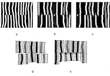
Figure 8.8.1: (a) Synthetic pattern of stripes indexed starting at the centre (b) and the left (c). The resultant shapes for (b) and (c) are shown in (d) and (e)... 118

Figure 8.9.1: Evenly spaced stripes projected onto image plane from surfaces 1 and 2... 119

Figure 8.10.1: Visualisation of horizontal occlusion... 120

Figure 9.3.2: Visualisation of scanned surfaces with variations in parameters... 124

Figure 9.3.3: Recording of planar wall... 126

Figure 9.3.4: Visualization of surface of planar wall...127

Figure 9.5.2: Indexed sets for template comparisons... 133

Figure 9.6.2: Recording of spherical surface...135

Figure 9.6.3: Visualisation of scanned spherical surface...136

(17)

Figure 9.9.1: The registration and fusion of patches... 143

Figure 10.3.1: Visualisation of car body part (left, Courtesy jaguar Cars Ltd.) and crumpled paper sheet (right)... 148

Figure 10.3.2: Indexing of image (a) using (b) Scanline, (c) Scan and Search and (d) Flood Fill methods...149

Figure 10.3.3: Concave Pair (left) and four categories (right)...150

Figure 10.3.4: Recorded image (left), disconnections (centre) and marked occlusions (right). 151 Figure A l: Display mode 1, showing polyhedral surface (detail)...183

Figure A2: Display mode 2, showing original recorded image (detail)...184

Figure A3: Display mode 3, showing indexed peak stripes (detail)...184

Figure A4: Display mode 4, showing indexed peak and trough stripes (detail)... 185

Figure A5: Display mode 5, showing point cloud projected onto Y-Z plane...185

Figure A6: Display mode 6, showing point cloud projected onto X-Z plane... 186

Figure A7: Display mode 7 showing trace array depicting N, S, E, and W directions of search. 186 Figure A8: Display mode 8, showing peaks (green), U disconnections (red), D disconnections (blue) and unknown connections (yellow) (detail)...187

Figure A9: Display mode 8, with the occlusion boundaries marked black (detail)... 187

List of Tables

Table 4.4.1: Mean error and standard deviation for Scan 10 out of 2 1 ... 43

Table 9.4.2: Mean error and standard deviation for planar surface... 129

Table 9.6.1: Measures for Flood Fill method on planar surface... 134

Table 9.6.2: Measures for scanned spherical surface... 136

(18)

Chapter 1: Introduction

Two distinct visual approaches towards the detailed and accurate representation of real objects

are computer graphics and computer vision. In this context "vision" refers to the automatic

recording of some properties of an object: photography records reflected light, and motion

capture records the position of the joints in a moving body. On the other hand "graphics" has no

such direct link with the real world; the output, such as a painting or a CAD drawing, is

rendered by hand or machine and may be continually modified to approach a representation of

reality. Many applications combine the two approaches, and this combination of graphics with

some form of automated vision can be seen in Canaletto's camera obscura paintings, Warhol's

screen prints, and in movies such as Disney's "Snow White" where cine film of actors (i.e.

"vision") is retraced and combined with traditional animation drawings ("graphics"). Computer

vision requires a considerable hardware investment in video capturing or motion sensing, but

the benefits over computer graphics rendering are significant. As [Watt, 2000] points out:

"Real world detail, whose richness and complexity eludes even the most elaborate

photo-realistic renderers, is easily captured by conventional photographic means".

This "richness and complexity" is important for both measurement and visualisation uses.

In the former category are such applications as reverse engineering, inspection and archiving

[Levoy et al., 2000] [GOM, 2004] [Yang et al., 1995], all of which require accuracy in the

measurements. In visualisation applications [Marek and Stanek, 2002] the viewer is less critical

of exact measurement, but will find a recording of a real object more intuitively lifelike than a

computer generated one due to unquantifiable nuances in the captured model.

The entertainment industry is particularly interested in acquiring the three-dimensional

model in real time, but at present some form of compromise is made, using both vision and

graphics. A standard method of producing an animated face is to map photographic images onto

a preformed computer model of a speaking head [Liu et a l, 2000]. This gives an impression of

true 3D vision, but will miss much of the appealing detail, and is a time-consuming process.

Recent research, especially in Structured Light Scanning and Stereo Vision, suggests the

possibility of producing a model of a complete surface area such as a human face within the

(19)

process provides synchronisation of face and voice, a conspicuous absence in photo-realistic

renderings.

1.1.

Methods of Recording 3D Surfaces

The general objectives of this research area can be usefully separated into two processes: firstly

to measure the three-dimensional position of points on the surface of a target object, and

secondly to order these points and thereby reconstruct a model of the surface as a mesh of

connected polygons. The former process, which we call “point acquisition”, is geometric,

defined by the spatial position of the system in Euclidean space; the latter process, which we

call “surface reconstruction”, is a graph topology issue whereby the acquired points are

connected in a graph of vertices and edges [Bondy and Murty, 1976]. The resulting 3D model

has an increasing number of industrial, medical and multimedia applications, which require

continual improvement in the speed of acquisition, accuracy of measurement and verity of the

reconstructed surface [Valkenburg and Mclvor, 1998]. In the field of Machine Vision using

video images, two main methods, Stereo Vision and Structured Light Scanning, compete to

fulfil these requirements.

Stereo vision, the system used for human sight, simultaneously records two spatially

related images and recognizes corresponding features in each scene [Marr and Poggio, 1979].

Knowledge of the geometric relation between the two images allows the three-dimensional

position of the features to be computed. The key to this system is the recognition of

corresponding features, and this task is known as the Correspondence Problem [Zhang, 1996].

If there is a dense map of these features then the target objects can be reconstructed accurately

and comprehensively, but if the object is a smoothly undulating form then features are difficult

to find and the surface is difficult to measure. A further problem is that the acquired points do

not explicitly provide a way of reconstructing the surface; forming the polygonal mesh from the

point set is itself the subject of considerable research effort [Curless and Levoy, 1996].

The Structured Light method projects a pattern of light onto the target surface, and a

sensor such as a video camera records the deformed light pattern reflected from the surface.

Here the correspondence problem is different: rather than finding the same feature in two stereo

images we need to find the correspondence between a projected pattern element and its

reflection from the target surface onto the sensor. If the spatial relationship between the camera,

(20)

featureless forms which Stereo Vision methods find difficult, and the projected pattern provides

a definable and controllable density which is not possible using feature recognition. However, if

the surface is not smooth, or is highly reflective, the coherence of the projected pattern may be

lost in the recorded image, and the surface will be difficult both to measure and to reconstruct.

A benefit of the Structured Light system is that the light pattern gives an order to the acquired

points, so that if the points are successfully derived then their connection sequence implicitly

follows. For example, if we project a grid pattern of dots, the derived points will be connected

in the same way as the projected dots, and a polygon mesh can be easily formed.

Therefore we see that the usefulness of these two methods is almost complementary:

Stereo Vision is applicable for densely featured surfaces, and Structured Light Scanning for

smoother surfaces. Unfortunately it is not necessarily possible to know in advance what type of

surface will be encountered, and which method will be preferable. Research is currently

attempting to extend the usefulness of each method into the domain of the other. For Stereo

Vision this means increasing the thoroughness of the search for common features and thereby

increasing the density of the point set; for Structured Light Scanning this means making sense

of the recorded image when the light pattern is severely deformed by the shape of the target

surface.

1.2.

Structured Light Scanning

Early Structured Light systems used a single stripe or spot of laser light to measure a small part

of the object in each scan [Rioux and Blais, 1989]. Now the availability of controlled light

output from LCD projectors allows the projection of a more complex pattern of light to increase

the area measured in a single scan. The classic Single Stripe scanning system provides the

profile of a "slice" through the target object. In order to build a model of the complete surface a

number of spatially related profiles must be scanned. To achieve this a sequence of scans is

captured. For each scan, the target object is moved in relation to the scanner, or the projected

stripe moves in relation to the object, the movement being controlled to the same resolution as

required by the scanning system. A system may require an accuracy of 1:20000 [Beraldin et a l,

2001].

(21)

captured as a sequence of stripes in a single frame [Valkenburg and Mclvor, 1998]. However, it

may be difficult to determine which captured stripe corresponds to which projected stripe, when

we attempt to index the captured sequence in the same order as the projected sequence. We

name this the Indexing Problem , and its solution will form the main subject of this thesis.

1.3.

Defining the Principal Research Questions

1.3.1. The Indexing Problem

Target Objecj

surface point s - (x,y,z) at stripe n

stripe n

Projecl or

LCD

CCD (reversed image) corresponding image point s'=(h,v).

[image:21.613.107.467.228.495.2]

at stripe n

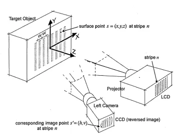
Figure 1.3.1: The structured light scanning system.

Figure 1.3.1 shows the basic Structured Light Scanning system, here using a sequence of

vertical, equally spaced stripes, shown grey for convenience. The vertical stripe sequence is

indexed, and the stripe with index n is shown as the dark stripe in the projector LCD. A point s

= (x,y,z) which is on the surface of the target object is illuminated by stripe n, and is recorded

on the camera CCD as point s' on the camera image plane. The position of s = (x,y,z) is given

by the scanning function scan(h,v,n) = ([x,y,z), where (h,v) is the position of the point s' as seen

(22)

a difficult task.

1.3.2. Coding Schemes

Because of these indexing difficulties, methods have been devised to encode the stripes, by

colour, stripe width, or by a combination of both. Coding schemes are discussed in detail in

Section 2.4.3, and reviewed by [Salvi et a l, 2004]. However, coding does bring disadvantages:

with colour indexing there may be weak or ambiguous reflections from surfaces of a particular

colour, and with stripe width variations the resolution is less than for a uniform narrow stripe.

This last problem can be addressed by projecting and capturing a succession of overlapping

patterns of differing width but this means that it is not possible to measure the surface in a

single frame. Single frame or "one-shot" capture is desirable because it speeds up the

acquisition process, and leads to the possibility of capturing moving surfaces. Moreover, most

of the coding schemes use a sequence which repeats, typically, every eight times, in which case

ambiguities are still possible. These coding options are illustrated in Figure 1.3.2 where at (1)

we see an uncoded pattern, at (2) a 3-colour coding, at (3) a pattern with varying stripe width,

and at (4) we see four binary patterns which are successively projected to give a Gray coding

scheme.

HI

H I

1 2 3 4

Figure 1.3.2: Stripe coding schemes.

The general strategy of this thesis is to determine how far the Indexing Problem can be solved

with uncoded stripes, where the correct order of stripes in the captured image is determined by

original algorithmic methods. It may then be appropriate to add a limited amount of coding to

solve some of the more intractable issues. A comparison will also be made with dot patterns,

(23)

1.3.3. The Principal Research Questions

From the two preceding sections it is now possible to pose the two main questions which will be

addressed in this thesis:

1. How can we correctly identify in the sensor a specific projected pattern element,

expressed as an index? This is the Indexing Problem.

2. How far can the Indexing Problem be solved using an uncoded projection pattern?

In order to answer these questions a number of investigation topics will be proposed, and we

begin by discussing some of the issues which will be encountered in this research.

1.4.

Choosing the Projection Pattern

Other researchers have proposed many types of pattern for Structured Light Scanning, such as

dots [Proesmans and Van Gool, 1998], grids, horizontal stripes and vertical stripes [Daley and

Hassebrook, 1998] [Guhring, 2001]. The patterns can be useful categorized into two types: two-

dimensionally discrete patterns such as dots or grids, and one-dimensionally discrete patterns

such as horizontal stripes or vertical stripes. The one-dimensionally discrete patterns are

continuous in their second dimension, so that vertical stripes are discrete from left to right, but

continuous from top to bottom. An advantage of this is that vertical stripes can be sampled

vertically at any point - in other words a portion of the vertical stripe will be present on every

pixel row. To sample discrete elements such as dots would require compliance with the

Nyquist-Shannon Rule [Nyquist, 1928] which states that the sampling frequency must be

greater than twice the highest frequency of the input signal. In spatial terms this means that in

the recorded image the spacing between dots would have to be greater than two pixels.

Given this clear advantage of stripes, it raises the question of whether there is any reason

for using two-dimensionally discrete patterns such as dots. Chapter 6 will show that knowing

(24)

provide confirmation of the index for that particular dot.

1.5.

Geometric and Topological Considerations

Both the geometry and the graph topology of the 3D model must be considered. The final goal

is a geometrically congruent model, i.e. an isometric representation in Euclidean space of the

target surface. However, because the scanned model will be discrete whereas the target surface

is continuous, a discrete approximation must be made, of a connected graph of vertices (see

Figure 1.6.1, right) with each vertex having a precise location in E3 space. If the system

parameters are correctly measured in the calibration process, and the graph of vertices is

correctly connected, then the resulting discrete model will be an ideal approximation.

If the system parameters are incorrectly measured, then this ideal approximation will be

deformed; the vertices will change their location and the distances between them will change;

therefore the model will lose its isometry and geometric congruence. This deformed shape will

still be topologically equivalent, because the transformation between the two shapes is

homeomorphic, i.e. bicontinuous and one-to-one.

Apart from by incorrect measurement of the system parameters, another way in which the

shape may change is by connecting the graph of vertices in a different way, thus changing the

combinatorial structure [Huang and Menq, 2002] of the graph. For instance, if a vertex is

connected to a different stripe path (see Section 7.6), the index will change and the 3D location

of that vertex will change (see Section 1.3.1). Finding the correct connection between vertices,

i.e. the combinatorial structure, is another way of expressing the task of the Indexing Problem.

In fact it may be useful to consider two separate tasks: the topological one of correctly

connecting the vertices, and then the geometric one of finding the E3 location of each vertex.

1.6.

Vertex Connections

In Figure 1.6.1 we see a detail of a recorded stripe pattern (left), the array of peaks at the centre

of each stripe for each row (centre), and the derived mesh of 3D vertices representing the target

(25)

vertices, and that the connections between their respective vertices are the same. Therefore once

the connections are established in the peak array, it becomes a simple task to connect the

vertices in the surface mesh. When thinking about how the Indexing Problem would be solved

for this example, two related tasks can be considered: to find the "connected path" for each

stripe, and to index the stripes in the correct sequence. Visually it is easy to see that there are

three stripes each with a connected path from top to bottom, and that they could be indexed

from left to right as stripes 1, 2 and 3.

Figure 1.6.1: Visualisation o f the stripe pattern.

We will investigate the ways in which the peak connections can be defined and

implemented. In defining these connections care is taken to comply with the common terms

used in graph theory such as "connectedness", "connectivity", "adjacency" and "paths".

Figure 1.6.2: Recorded image fro m structured light scanner (part).

Figure 1.6.2 shows part of a typical image recorded by a Structured Light Scanner. The

projected pattern of evenly spaced, vertical white stripes appears to be deformed by the shape of

(26)

stripes, but there are some areas where either the stripe is missing (around the ear) or there is

ambiguity over which direction it should take (to the right of the nose). There may also be

situations where we trace an apparently continuous stripe where there is in fact a disconnection

(possibly under the nose). In this situation the nose is occluded from the camera viewpoint, and

the shadow to the left of the ear is occluded from the projector viewpoint.

The investigations into connections will use this intuitive visual approach as a starting

point for some of the automatic algorithms, and will also look at methods of overcoming the

problems set by occlusions.

1.7.

Ambiguous Interpretation

Figure 1.7.1 shows at (a) a hand-drawn, hypothetical image from a scanner. Two attempts to

index the stripes (using colour as a guide) are shown at (b) and (c), with a visualisation of their

resulting surfaces at (d) and (e), where the coloured stripes are superimposed onto the surfaces

for demonstration purposes. In (b) we assume that a complete stripe is present at S.

[image:26.613.105.483.380.640.2]

d e

(27)

The indexing of the rest of the image follows from there and, in order to make sense of the

stripe pattern, two horizontal steps are assumed in the areas marked with “x”. A similar process

occurs for version (c), this time with the assumed complete stripe S being at the extreme left.

Once again a horizontal step is assumed, this time at the centre. The visualisations at (d) and (e)

show the horizontal steps which are assumed in order to solve the Indexing Problem. This

hypothetical example suggests that there will be cases where apparently "connected" stripe

elements are in fact "disconnected", and also that if this area is the full extent of the image it

may be impossible to decide which interpretation is correct.

1.8.

Definitions and Identification of Occlusions

There are a number of potential reasons why there may appear to be a disconnection, an

ambiguity or an incorrect connection in the recorded stripe patterns. One likely source is

occlusions [Park et al., 2001], where part of the surface is hidden from either the projector (the

shadow on the wall in Figure 1.6.2) or the camera (the hidden side of the nose). It may be

possible to improve the success of the indexing algorithms by better understanding the

contribution of occlusions. In Figure 1.6.2 we know, because the object is a face, that there is an

occlusion at the nose which will then give us clues as to what course the stripes are likely to

take. However, an automatic algorithm will not have this prior knowledge, unless it is included

within the program; but it may be possible to categorize occlusions and predict their likely

affect. One major investigation topic will look closely at how the relationship between projected

stripes and their recorded image is affected by the presence of occlusions, and provide

definitions and categorization of occlusions which will be useful for this and other work.

1.9.

Geometric Constraints

Some questions arise which relate vertex connections with the geometric setup of the system.

The recorded image, such as in Figures 1.6.2 and 1.7.1, includes topological and geometric

information, both of which are required to calculate the parameters of the scanning function

scan(h,v,n). Here "topological" is used in the sense of "graph connectivity in 2D", and this

connectivity is used to find the index n for all stripes; accurate geometric measurement of the

(28)

possible to use this duality to answer questions in the topological graph by referring to the

Euclidean space, and vice versa.

For instance, in Figure 1.7.1 (c) the three centre stripes are assumed to be "disconnected",

split by an invisible horizontal step; and yet it may be possible to calculate geometrically that

any such step would require the stripes above and below the step to be differently spaced. This

is shown in Figure 1.9.1 (left) where the spacing between the stripes above the step is w' units

and the spacing below the step is w" units. This would then prove that the assumed topology, of

a horizontal step, is impossible if there is no change in spacing.

Step

ir

Figure 1.9.1: Horizontal step (left), and lateral translation (right).

Also, we notice in Figure 1.6.2 that the stripes on the ear lobe are continued on the back wall,

but much lower down in the image. There is a shadow occlusion between the head and the wall.

Can we constrain the system so that when a stripe stops due to an occlusion it will always be

picked up again in the same horizontal line? (as in Figure 1.9.1 right). It may be that we can set

up the apparatus in such a way that we can answer these questions and thereby improve the

reliability of the connection algorithms and other indexing methods.

A concept which is commonly used in Stereo Vision is that of Epipolar Geometry,

whereby a spatial constraint is imposed so that corresponding pairs of features must be

somewhere along known epipolar lines, thus reducing the Correspondence Problem to a one

dimensional search along that line [Faugeras et al., 1993]. Epipolar Geometry (see Chapter 6,

Section 6.3) will be used to investigate the condition described in Figure 1.9.1 (right), and also

(29)

1.10. Definitions of Success

While conducting these investigations we will be mindful of how best to measure the success of

the outcomes. In some applications, such as industrial testing, it may be preferable to have a

smaller surface area with a high degree of confidence in the accuracy of the model; in other

areas, such as computer animation, it may be acceptable to have a number of errors but with as

large a patch of surface as possible. A further problem will be how to test for accuracy. It will

be necessary to have some kind of template object, with independent knowledge of its

dimensions, to test against; but if we are to test a complex surface, as we must, how will we

independently measure that surface?

In some cases, such as the hypothetical pattern in Figure 1.7.1, it may be impossible by

our primary methods to determine which surface representation is true, or which is more likely.

At this point it will be necessary to ask whether our initial strategy, of using an uncoded stripe

pattern, is feasible. Further strategies may be considered, such as a categorization of the surface

by curvature or Fourier analysis, implementation of a limited colour coding scheme, or

assuming that the system is scanning a specific shape, say a face or a production line item,

which would have the advantage of including prior knowledge in the algorithms.

Definitions and descriptions of the methods used in this thesis will be given in Chapter 5.

1.11. Summary of Investigation Topics

From the above discussion five primary investigation topics are educed:

Inv 1. The use of geometric constraints, and in particular Epipolar Geometry, to

alleviate the Indexing Problem.

Inv 2. A comparison between the benefits of two dimensionally discrete patterns

such as dots, and patterns such as stripes which are discrete in one

(30)

the boundaries of the target surface.

Inv 4. Understanding the relevance of occlusions to the Indexing Problem.

Inv 5. Testing the Success of the Indexing Methods.

The research methods and strategy employed for these investigations are discussed in Chapter 3.

1.12. Original Contributions

This thesis makes original contributions in regard to geometric constraints, connectivity,

measures of success, and occlusions. The contributions made are described at the start of each

relevant chapter, and summarised in the Conclusions.

We take the popular methods using Epipolar Geometry and Rectification and adapt them

to investigate the use of Dot and Stripe Patterns in Structured Light Scanning. In particular we

introduce the Unique Horizontal Constraint and determine how far this can be successfully

used to solve the Stripe Indexing Problem. As far as is known, this method has not been used by

previous researchers.

Issues related to the connectivity of the vertex graph include definitions of N-, S-, E- and

W-Neighbours, leading to definitions of Stripe Paths and Neighbourhoods. These types form

the basis of descriptions of Patches, and are used as Patching Conditions in the novel

algorithms which have been designed to successfully index the stripes. These novel indexing

algorithms comprise Scanline, Scan and Search and Flood Fill methods, which adapt and

extend existing search methods used in Pattern Recognition and Segmentation applications.

Here we also pose the Size v. Accuracy Question: "For a given scanning application, what is

the relative importance of indexed patch size compared with indexing accuracy", and this

question must be addressed by the application designer.

In order to measure the success of these algorithms, all the indexing methods are executed

using a test object, which is compared to a hand-produced template result. Three novel

measures: total patch size, accurate patch size and indexing accuracy are used to evaluate the

(31)

To overcome the problems caused by occlusions, we make specific definitions which

relate occluded areas on the target surface to the resulting recorded image: Near Occlusion

Points, Far Occlusion Points, Projector Occlusion Points and Camera Occlusion Points.

From these definitions four boundary types are categorized: the Concave Pair, the Contour

Single, the Concave Tuple and the Contour Tuple. The investigation then looks specifically at

how Concave Pairs can be identified in the recorded image, and thence designs a novel

algorithm to detect and m ark the occlusion boundary. This is added to the Patching

Conditions, giving improved levels of indexing accuracy. These investigations relate to

occlusions which are not horizontal. In addition, a theoretical instance has been designed which

shows that it is possible to have exactly the same spacing between stripes, above and below a

horizontal occlusion (or step). This means that spacing between stripes cannot be readily used

as an indicator of the presence of a horizontal occlusion.

1.13. Overview of the Thesis

The objective of the thesis is to investigate the two principal research questions:

• how can we correctly identify in the sensor a specific projected pattern element,

expressed as an index (this is the Indexing Problem), and

• how far can the Indexing Problem be solved using an uncoded projection pattern?

In Chapter 2 we look at prior work in the field of surface measurement, particularly those areas

which use triangulation rangefinding. This covers techniques such as laser scanning and coded

structured light scanning. Particular problem areas are reviewed, such as occlusion handling,

connection algorithms and calibration methods, and work in the associated discipline of Pattern

Recognition is described. Applications such as heritage replication, reverse engineering,

medical uses and multimedia productions are listed.

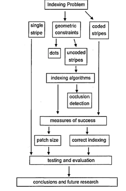
The strategy, methods and investigations undertaken in this thesis are described in

Chapter 3. A brief outline is given of the five investigation topics: geometric constraints, the

comparison between dots and stripes, the connection algorithms, occlusions, and testing

(32)

process is shown as a flow diagram incorporating the investigation topics.

Chapter 4 gives a detailed account of the Single Stripe Scanner which has been built as

part of the investigations. Many of its processes are used and adapted by the Multiple Stripe

Scanner, and the results obtained provide a useful comparison and measure of the success of the

whole project. Partly using the data types and methods from the Single Stripe Scanner, Chapter

5 describes in detail the data structures which are used in the thesis, the solving of the scanning

functions, and the problems associated with data acquisition and processing. The techniques

used for system calibration are also described.

The three following chapters concentrate on the main investigation topics: geometric

constraints, indexing algorithms, and occlusion issues. In Chapter 6 the principles of Epipolar

Geometry are explained, how they are implemented in relation to Stereo Vision, and methods

for adapting the techniques in Structured Light Scanners. There follows a comparison between

the benefits of using dot and stripe patterns using epipolar constraints. In Chapter 7 definitions

of connections between stripe elements are given, some of which are analogous to work in

Pattern Recognition. Initial algorithms are designed to search through the graphs and find

correct indices, resulting in patches of indexed surface. A particular problem is identified: that

of incorrect indexing due to occlusions. Chapter 8 gives definitions of camera and projector

occlusions, and the ways in which occluded areas are formed. From these definitions, methods

are designed to mark occluded areas in the recorded image, and thence the indexing algorithms

are revised.

Chapter 9 tests the processes, and gives comparative results of the success achieved with

different algorithms, which are modified in ways suggested by the investigations. In Chapter 10

conclusions are drawn from the investigations, and suggestions are made for further work based

(33)

Chapter 2: Prior Work on Surface Measurement

Surface measurement can be broadly split into two categories: contact and non-contact methods.

Here we are concerned with non-contact techniques which are generally known as

“rangefinding” [Jarvis, 1983][Karara, 1989][Blais, 2004], and within that domain we make a

further separation between image-based methods, interferometry, time-of-flight, and

triangulation methods.

2.1.1. Image-based methods

Image-based methods take a collection of recorded images of the target object and by various

processes calculate a 3D rendition of the target object. A technique of [Wood et al., 2000] and

[Wilburn et al., 2002] uses "surface light fields" which invert the usual ray-tracing methods to

produce a rendition of the specular surface of the object.

It is also possible to estimate spatial position from the optical flow [Vedula et al., for

publication 2005] [Verri and Trucco, 1998] of a target object through a sequence of images

[Zhang and Faugeras, 1992], [Koch et al., 1998]. The optical flow of the scene can be used to

separate the target object from the background [Iketani et al., 1998] [Ngai et al., 1999] [Bregler

et al., 2000], to recognize hand gestures [Jeong et al., 2002], and facial motion [Reveret and

Essa, 2001]. The supersampling which the recording of a moving object provides also allows

for the development of super-resolved surface reconstruction [Cheeseman et al., 1994]

[Cheeseman et al., 1996].

2.1.2. Interferometry and other wave analysis techniques

Interferometry measures differences between two phase-separated beams of light, as devised in

the classic Michelson-Morley experiment [Michelson and Morley, 1887]; moire and fringe

projection can be used to measure very small surface depths [GOM, 2004][Maruyama and Abe,

(34)

Time-of-flight systems transmit a signal onto the target surface, and a sensor positioned close to

the transmitter records the time taken between transmission and sensing. Because of the short

times involved, time-of-flight systems generally work over a large distance, although techniques

such as single photon counting [Pellegrini et al., 2000] [Wallace et al., 2002] can bring the

distances down to less than one metre.

2.2.

Triangulation Rangefinding

The term “triangulation” as used here relates to the concept of trigonometric measurement,

where two angles and two vertices of the triangle are known, and thence the position of the third

vertex can be calculated. We will look at two topics which comprise the bulk of the research

activity, Stereo Vision and Structured Light Scanning. In addition, calculation of depth using

focus as a parameter [Subbarao and Liu, 1998] is a well researched area, especially in low-

resolution applications such as robotics [Nayar et al., 1995].

2.3.

Stereo Vision Techniques

As described in Section 6.3, the Stereo Vision process records two spatially related images of

the same scene, finds corresponding features in the two scenes, and thence calculates the

position of that feature in the system space. Where the same techniques are used for both Stereo

Vision and Structured Light methods, they will be described below, but early work in this field

was done by [Koenderink and van Doom, 1976] and [Marr and Poggio, 1979]. Research has

also investigated the use of multiple cameras [Chen and Medioni, 1992] [Faugeras et al., 2002],

and specifically three-camera systems [Blake et a l, 1995].

The finding of corresponding features in the two scenes, known as the Correspondence

Problem, is considered to be a difficult task [Zhang, 1996], and the similar problem for

(35)

2.4.

Structured Light Scanners

2.4.1. Single Stripe Scanners

The earliest successful light projection rangefinders used laser beams, usually in a single stripe

of light. Lasers provide a focusable, high level of illumination in a small package; in

comparison slide projectors or other white light systems are cumbersome and difficult to

control. The stripe of light is cast onto the target object and the recorded image is used to

calculate the depth of the profile where the light stripe intersects the target surface. To produce a

sequence of profiles which can be used to model a complete surface, either the stripe has to be

moved in relation to the target object, or the target object moved in relation to the projected

stripe. Either way, this must be done in a spatially controlled manner.

At the National Research Council of Canada (NRC) [Rioux and Blais, 1989] modified a

standard camera lens by inserting a mask between two lens elements which produced a double

image on the CCD sensor. The laser was projected via a rotating mirror controlled by a high

precision galvanometer. An RMS deviation in the range axis was 40pm for a 300 mm volume

was reported. [Beraldin et al., 1992] developed a method to calibrate the synchronised scanner

and compare experimental results with theoretical predictions. The calibration method used a

planar wedge with fiducial markings to provide data for a look-up table array, which would then

map to collected data for the target object. Estimates were then made of the range errors, and it

was found that the limiting factor was the laser speckle impinging on the CCD, which noise far

outweighed that contributed by electronic and quantization noise.

The NRC scanners produced a high accuracy, reported to be in the order of 40pm;

however, they required precisely engineered moving parts to scan through the range plane.

Many alternatives have been developed which require less complex mechanisms.

The work described above by the National Research Council of Canada led to an

important and prestigious direction for projected light scanners: heritage applications. The

Digital Michaelangelo Project [Levoy et al., 2000] used single stripe scanners to produce

surface models of many of Michaelangelo's sculptures, including the 5m tall statue of David, to

an accuracy of 1mm. From this model a copy of the sculpture can then be made [Beraldin et a l,

2001] using computer controlled milling machines, to replace the original statue in difficult

environments (susceptibility to pollution or vandalism, for instance). In the Digital

Michaelangelo Project a colour image was recorded alongside each scan, so that the modelled

(36)

scanner, where the target object is rigid and often has a diffuse surface. Single stripe scanning

technology has now produced a range of stable, popular products for these rigid surface

applications. Research has moved to structured light scanning, which captures more than one

profile, by projecting a more complex pattern of light.

2.4.2. Solutions using fixed camera/source systems

At the Machine Vision Unit at the University of Edinburgh, [Trucco and Fisher, 1994] used a

laser stripe projection in a fixed relationship with two CCD cameras, the target object being

moved laterally using a microstepper motor to scan along the X-axis. Using two cameras

reduced spurious results caused by specular reflection and occlusions. A look-up table would be

created using a stepped ramp as a calibration object, which would then map to the target object

data. Standard deviation results using the calibration object were approximately 0.1 mm,

depending on the specularity of the surface. The advantage of using a calibration matrix is that

non-linearity, especially that caused by the spherical geometry inherent in the system, does not

have to be overcome using mathematical calculations. However, calibration can be a time

consuming process which is not suitable where more immediate results are required.

[McCallum et a l, 1996] developed a hand-held scanner, also using a fixed relationship

between the laser and the camera to project and receive the light stripe. In this case the stripe

moves freely across the object as the apparatus is manually operated. The position of the

apparatus in world co-ordinates is given by an electromagnetic spatial locator. Inaccuracies in

the spatial locator reduce the resolution of this system to 1.5 mm at a range of 300 mm, and are

a major drawback to its widespread use. This scanner has been built as a commercial product

[McCallum et al, 1998]:

When multiple stripes or other sequenced patterns are used, to increase the area scanned

in a single video frame, the Indexing Problem occurs, and the following research has been

(37)

2.4.3. Coding schemes

As described in Chapter 1, Structured Light Scanners [DePiero and Trivedi, 1996] project a

pattern of light, such as dots, grids or stripes, in order to increase the area of surface captured in

one recorded image. To solve the Indexing Problem, akin to the Correspondence Problem in the

Stereo Vision field, many codification strategies have been proposed and implemented, and are

reviewed by [Salvi et a l, 2002], These include binary coding, n-ary coding, De Bruijn

sequences and colour coding.

Binary coding schemes [Daley and Hassebrook, 1998] [Valkenberg and Mclvor, 1998],

project a pattern of different width stripes so that the pattern can be successfully indexed.

Because the stripes have different widths, the highest possible resolution will not be achieved at

the widest stripes, and therefore further patterns are projected which overlap each other and

result in a successfully indexed pattern with a uniform resolution. The disadvantage of this is

that a number of frames, fourteen for the Daley-Hassebrook method, nine for the Valkenberg-

Mclvor method, are required for each complete scan. Valkenberg and Mclvor report the

importance of using substripe estimation and incorporating lens distortion into the projector

model.

[Rocchini et al., 2001] extended their binary coding by incorporating a colour scheme of

red, green and blue stripes, although this still requires nine frames to complete the scan. [Hall-

Holt and Rusinkiewicz, 2001] have proposed and implemented a coding scheme using coloured

stripes which produces a surface model from one single recorded image. The choice of pattern

has been optimized for moving scenes, and the results produce scans without the need to

calibrate object motion. However, the target object must move fairly slowly in order to avoid

erroneous temporal correlations. [Zhang et al., 2002] also project a pattern of coloured stripes,

and thence detect an edge with a triple colour value (r,g,b). The correct indexing is sought using

a multiple hypothesis technique, which admits the possibility of more than one solution. A score

is then given for each possible solution, based on a match between the colour triple in both the

projector scanline and the camera scanline. Importantly, this assumes that the system is

constrained such that the displacement of each point must be along a scanline, according to the

constraint suggested by [Faugeras, 1993]. Results show that this method is able to correctly

model disconnected components, where no surface connectivity exists, although artefacts still

occur due to false edges at the boundaries. Another one-shot colour coding scheme has been

developed by [Sinlapeecheewa and Takamasu, 2002] using six colours in an eleven stripe

(38)

here again the results are given only visually, and state the future objective of processing slowly

moving objects.

A method employing two successive patterns of uncoded stripes, one vertical and one

horizontal, has been proposed by [Winkelbach and Wahl, 2002]. Here the spacing between

stripes is used, along with the comparison between the horizontal and vertical patterns, to create,

at each node of the combined grid pattern, a surface normal. These normals are then used to

create the surface model. Results with standard commercial cameras and projectors report a

standard deviation of the surface normals of 1.22 degrees.

2.4.4. Combining Stereo Vision with Structured Light

In order to model more complex 3D scenes, with a number of unconnected objects, [Scharstein

and Szeliski, 2003] have combined the techniques of stereo vision and binary stripe projection.

Using two cameras and one projector, they report disparities of between 10 and 20 percent on

these difficult scenes. [Devemay et a l, 2002] have produced a one-shot scanner using a camera

and projector; a white noise pattern is projected, and a single video image captured. The

correspondence problem is solved using standard correlation-based stereo algorithms. Reported

limitations in this system are dealing with occlusions, highly-textured surfaces, and surfaces

which are almost normal to the camera view.

2.4.5. Estimating the centre of the stripe in the recorded image

A comparison of eight algorithms to find the centre of the light stripe has been made by [Fisher

and Naidu,1996]. It is assumed that the light incident upon the target object follows a Gaussian

distribution, although it is noted that the sensing system of the CCD will affect the fidelity with

which this distribution is recorded. Of particular interest are the "Centre of Mass" algorithms,

which calculate the arithmetic mean of the brightest pixel and the two (COM3), four (COM5)

and six (COM7) adjacent pixels. The COM3 algorithm performs poorly, but the other seven

produce empirical results in the same range. [Curless and Levoy, 1995] devised a spacetime

method which analysed successive adjacent scans in order to correct reflectance, shape and laser

(39)

to the existing hardware were required. This subject area of comparing and interpreting data in

adjacent frames is an important topic for research. An alternative to using the Gaussian profile is

to use the transitions between stripes [Mclvor, 1997] which may be a more reliable method for

multiple stripe systems. [Mclvor and Valkenburg, 1997] proposed three substripe estimation

methods: polynomial fitting using stripe indices, boundary interpolation using an edge detector,

and sinusoidal fitting with six harmonics. Tests were executed using a planar surface, which

gave the best results (the lowest standard deviation) to the sinusoidal fitting method.

2.4.6. Laser speckle phenomena

Laser speckle can be considered as either a source of unwanted noise or as a useful measuring

entity. Laser speckle is caused by coherent light of a specific wavelength continually hitting the

same microscopic particle (and a discrete number of its neighbours) and producing an

interference pattern along the line of sight. With incoherent light the wavelengths are constantly

changing so that an averaging effect is produced at the sensor, which sees a comparatively

uniform reflectance. Laser speckle reduces the predictability of the beam profile and limits the

accuracy of range measurements [Beraldin et al., 1992]. The light stripe data can be operated on

by filtering convolutions [Becker, 1995] which blur the stripe in a Gaussian form, although the

wider stripe can cause problems for multi-stripe applications. [Hilton, 1997] has used laser

speckle in a constructive way to measure the roughness of a surface.

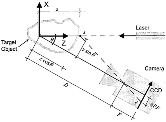
A series of experiments conducted by [Clarke, 1994] pointed a light beam along the axis

of a CCD camera, and placed a sheet of white paper at measured intervals between the light

source and the camera lens. Results using laser light and white light sources showed maximum

errors for white light of 0.199 pixels, and for a series of lasers of between 0.389 and 1.292

pixels. Clarke concludes that the coherence of lasers has a highly significant effect in degrading

the location of the laser target.

2.5.

Calibration

Calibration of a triangulation rangefinder requires the determining of two sets of parameters:

intrinsic and extrinsic. Early work on the geometric measurements was undertaken by [Brown,

(40)

onto the sensor. The extrinsic parameters are those which set the spatial position of the

projector, cameras and any other elements of the apparatus. Both automatic and manual

methods have been devised, some using calibration charts or objects, others deriving the

parameters from the target object themselves. [Trucco and Fisher, 1994] calibrated a single

stripe scanner by sliding a ramp of known dimensions across the stripe and thence deriving a

look-up table of depth values for all parts of the recorded image. This provides both intrinsic

and extrinsic parameters, but requires considerable preparation before each scanning session.

[Shen and Menq, 2002] used a calibration plane as a target object, and projected a grid pattern