Stability Analysis for a Discrete SIR Epidemic Model with Delay and General Nonlinear Incidence Function

(1)

ISSN Online: 2152-7393 ISSN Print: 2152-7385

DOI: 10.4236/am.2018.99070 Sep. 18, 2018 1039 Applied Mathematics

Stability Analysis for a Discrete SIR Epidemic

Model with Delay and General Nonlinear

Incidence Function

Aboudramane Guiro

*

, Dramane Ouedraogo, Harouna Ouedraogo

Département de Mathématiques, UFR des Sciences et Techniques Université Nazi Boni de Bobo-Dioulasso & LAboratoire de Mathématique et d’Informatique (LAMI), Bobo-Dioulasso, Burkina Faso

Abstract

In this paper, we construct a backward difference scheme for a class of SIR epidemic model with general incidence f. The step size

τ

used in our dis-cretization is one. The dynamical properties are investigated (positivity and the boundedness of solution). By constructing the Lyapunov function, the general incidence function f must satisfy certain assumptions, under which, we establish the global stability of endemic equilibrium when R0>1. The global stability of diseases-free equilibrium is also established when R0≤1. In addition we present numerical results of the continuous and discrete mod-el of the different class according to the value of basic reproduction number

0

R .

Keywords

Discrete Model, Delay, Lyapunov Functional, Nonlinear Incidence, Backward Difference Scheme, Local Stability, Global Stability

1. Introduction

In certain epidemiological modeling, the population is generally divided into three classes which are susceptible represented by S, infected individual represented by I and recovered individual represented by R. This kind of ma-thematical model is noted SIR. Recently, many authors have studied the dynam-ical behavior of epidemic models (see [1] [2] [3] and references therein). There are two kinds of mathematical models: The continuous-time models described by differential equations, and the discrete-time models described by difference equations. The simplest forms of these models are Ordinary Differential Equations How to cite this paper: Guiro, A.,

Oue-draogo, D. and OueOue-draogo, H. (2018) Sta-bility Analysis for a Discrete SIR Epidemic Model with Delay and General Nonlinear Incidence Function. Applied Mathematics, 9, 1039-1054.

https://doi.org/10.4236/am.2018.99070 Received: July 16, 2018

Accepted: September 15, 2018 Published: September 18, 2018

(2)

DOI: 10.4236/am.2018.99070 1040 Applied Mathematics (ODEs) [4] [5]. In [2], a discrete delay model is given to account for transmis-sion by vectors (e.g. mosquitoes), where the delay

τ

is used to account for a latent period in the vector. Allowing the vectors latency periods to vary accord-ing to some distribution gives a model with a distributed delay [6].

The delay appears in the incidence term which is typically the only non-linearity, and is therefore the “cause” of all “interesting behavior”. Various forms have been used for the incidence term, both for ODEs and for delay equa-tions. Common forms include mass action

β

SI [6] [7] [8], saturating incidence

1

I S

cI

β

+ [9] [10], and standard (or proportional) incidence

SI N

β

[4]

(

N S I= +

)

_{. Changing the form of the incidence function can potentially}

change the behavior of the system.

In this paper we study the discrete mathematical model which result from the continuous-time model presented and study in [11] by C. Connell McCluskey. From this we use the general incidence term

( )

(

)

0 ,

h

j n n j k j f S I

β

=

∑

, where h>0

is a time delay. We choose the constant

β

so that

( )

0 1

h j= k j

=

∑

. The discrete model is obtained by using the backward Euler method.

The studied of discrete epidemic models is motivate by the fact that there oc-cur situations such that constructing discrete epidemic models is more appro-priate approach to understand disease transmission dynamics and to evaluate eradication policies because they permit arbitrary time-step units, preserving the basic features of corresponding continuous-time models [12]. Furthermore, this allows better use of statistical data for numerical simulations due to the reason that the infection data are compiled at discrete given time intervals. For a dis-crete epidemic model with immigration of infectives, Jang and Elaydi [13]

showed the global asymptotic stability of the disease-free equilibrium, the local asymptotic stability of the endemic equilibrium and the strong persistence of susceptible class by means of the nonstandard discretization method. In he’s re-cent work, using a discretization called “ mixed type” formula in Izzo and Vec-chio [14] and Izzo et al. [15], Sekiguchi [16] obtained the permanence of a class of SIR discrete epidemic models with one delay and SEIRS (Suscepti-ble-Latent-Infected-Recovered-Susceptible) discrete epidemic model with two delay if an endemic equilibrium of each model exists.

(3)

DOI: 10.4236/am.2018.99070 1041 Applied Mathematics

2. Discrete Mathematical Model

In this section we describe the discrete mathematical model derived by the con-tinuous time model study in [11], by C. Connell McCluskey. This continuous time model is given by:

( ) (

)

( ) (

)

(

)

0

, d ,

,

h S h

I R

S B S k f S I

I k f S I I

R I R

τ

µ β τ τ

β τ τ µ γ

γ µ

 = − −

 

 = − +



 = −



∫

  

(1)

where Iτ =I t

(

−τ

)

.

1) A population is divided into susceptible, infectious and recovered classes with sizes S S t=

( )

_, I I t=

( )

_and R R t=

( )

_{respectively.}

2) B is the recruitment of new individuals, it is into the susceptible class. 3) µS, µI and µR denote respectively the death rates of susceptible,

infec-tious and recovered class.

4) The total exit rate for infectious is µI +γ , which, for biological reasons we

assume is at least as large as µS; that is, µI+ ≥γ µS.

5) The incidence at time t is β

∫

₀hk

( ) (

τ f S I, τ

)

dτ where the maximum delay 0

h> _,_k_{is a Lebesgue integral function which gives the relative infectivity of}

vectors of different infection ages. We choose

β

_{so that}

_∫

₀hk

( )

τ τd =1_{. It is}

assumed that the support of k has positive measure in any open interval having supremum h so the interval of integration is not artificially extended by con-cluding with an interval for which the integral is automatically zero.

The form of the function f is of fundamental importance. In this paper we use a general incidence function used in one of he’s discrete version. So we use as-sumption:

H1 f is a non-negative differentiable function on the non-negative quadrant. Furthermore, f is positive if and only if both arguments are positive.

H2 for all

( )

_{S I}_, 2

+

∈_ f S

( )

,0 = f

( )

0,I =0_.

The partial derivative of f are denoted by f1 and f2 from the first and second variable.

H3

(

) (

0

)

2

, j ,0

n n n

f S I ≤ f S I _{for all}_n_.

H4

(

)

(

)

* * _* _*

1 1

, , j

n n

f S I _S _I

S I

f S+ I + + +

≤ ≤ for all n.

Now, we use the backward Euler difference scheme to discretize the model (1). The time step size of our discretization is one. Thus, we obtain the following discrete SIR epidemic model with nonlinear general incidence given by:

( )

(

)

( )

(

)

(

)

1 1 1 1

0

1 1 1 1

0

1 1 1

,

h

j

n n S n n n

j h

j

n n n n I n

j

n n n R n

S S B S k j f S I

I I k j f S I I

R R I R

µ β

β µ γ

γ µ

+ + + +

=

+ + + +

=

+ + +

 ₋ _{= −} ₋

 

 ₋ ₌ ₋ ₊

 

− = −



∑

(4)

DOI: 10.4236/am.2018.99070 1042 Applied Mathematics where _Ij₌_{I t j}

(

₋

)

_.

Since R does not appear in the first and second equations of system above, it is sufficient to analyses the behavior of solutions of the following system:

( )

(

)

( )

(

)

(

)

1 1 1 1

0

1 1 1 1

0

,

h

j

n n S n n n

j h

j

n n n n I n

j

S S B S k j f S I

I I k j f S I I

µ β

β µ γ

+ + + +

=

+ + + +

=

 ₋ _{= −} ₋

  

 ₋ ₌ ₋ ₊



∑

(3)

The constants B, , ,µ µ γS I and the relation between this constants are given

above. In the discrete model the incidence function at time t is

( )

(

1 1

)

0 ,

h

j n n

j k j f S I

β + +

=

∑

,

where the maximum delay h>0_{. Let} E S I

( )

, be a equilibrium point model of (3) so we have,

( )

( ) (

)

, 0

S I

B S f S I

f S I I

µ β

β µ γ

− − =

 

− + =

 (4)

By adding the equations of system above we get

(

)

0

S I

B−µ S− µ +γ I=

(

I

)

_.

S

B I

S − µ_µ +γ

⇒ = (5)

Let E0 and E* be respectively disease-free equilibrium and endemic equi-librium point of model (3). The disease-free equiequi-librium correspond to the case where the infectious class is nil

(

I=0

)

_{. Thus, we have}E₀=

(

S₀,0

)

_{; with}

0

S

B S

µ

= _{. The endemic equilibrium} _E*_{is given by:} _E*₌

(

_{S I}*_, *

)

_{; with}

(

)

*

* I

S

B I

S = − µ_µ+γ _.

Proposition 2.1. The basic reproduction number is given by 2

( )

0 0

I

f E R =β_µ _γ

+ . Proof: The Jacobian matrix of system (3) at equilibrium E0 is define by:

( )

0

1 0 2 0

.

( )

S E

I

f E f E

J

f E f E

µ

β

µ γ

− − − 

= _ ₋ ₊ _

  (6)

Let

( ) (

)

2 0 I ,

A=β E − µ +γ ₍₇₎

( )

2 0 et I .

M =βf E D=µ γ+ ₍₈₎

Thus, we have:

1 0

R ₌MD− ₍₉₎

( )

2 0

0 .

I

f E R =β_µ _γ

(5)

3. Basic Properties

We suppose that initial condition of system (3) satisfy:

( )

0 0 and

( )

for all

[

,0 ,

]

S > I θ = Φ θ θ∈ −h ₍₁₁₎

where Φ ∈ = C

(

[

−h,0 ,

]

+

)

, the space of continuous functions from

[

−h,0

]

to + equipped with the sup norm: Φ =supθ∈ −[ h,0]Φ

( )

θ . Standard theory of functional differential equations [17] can be used to show that the solution of (1) exist and are differentiable for all t>0_{. We assume any initial condition for}

which the disease is initially present satisfies I

( )

θ >0_{for all} θ ∈ −

[

h,0

]

_.

Lemma 3.1. Let

(

S In, n

)

be a solution of system (3) with initial condition

(11), then we have Sn>0 and In>0 for all n.

Proof: Assume that Sn>0 and In>0. From system (3) we have the

fol-lowing system:

(

)

( )

(

)

(

)

( )

(

)

1 1 1

0

1 1 1

0

1 ,

1 , .

h

j

S n n n n

j h

j

I n n n n

j

S B S k j f S I

I I k j f S I

µ β

µ γ β

+ + +

=

+ + +

=

 + = + −

  

 + + = +



∑

(12)

By using second equation of system above and the fact that In>0, we have,

1 0

n

I + > . So In> ∀ ∈0, n . From the non-negativity of Sn+1 we used the as-sumption H4. Thus, S In, n>0 for all n.

Lemma 3.2. Any solution

(

S In, n

)

of system (3), with initial condition (11)

satisfy

(

)

limsup n n .

n _S

B

S I _µ

→+∞

+ ≤

Proof: Let Nn =Sn+In and Nn+1=Sn+1+In+1; for biological reasons we as-sume is at least as large as µS; that is, µI + ≥γ µS.

By adding the different equation of system (3) we get:

(

)

(

)

1 1 1

1 1

1

n n S n I n S n S n S n n S n

N N B S I

B S I

B N

µ µ γ

µ µ

+ + +

+ +

+

− = − − +

≤ − −

≤ − +

≤ −

1 1

SNn Nn Nn B

µ ₊ + ₊ − ≤ ₍₁₃₎

1 1 1

limsup S n n n limsup S n

n→+∞µ N + +N + −N = n→+∞µ N + (14)

1

lim sup S n n→+∞µ N+ B

⇒ ≤

1

limsup n .

n _S

B

N + _µ

→+∞

⇒ ≤ ₍₁₅₎

Hence, we have

(

)

limsup n n .

n _S

B

S I _µ

→+∞

+ ≤ ₍₁₆₎

(6)

DOI: 10.4236/am.2018.99070 1044 Applied Mathematics 1) When R0<1, then model (3) has only a unique disease-free equilibrium

(

0

)

0 ,0

E = S _.

2) When R0>1, then model (3) has only a unique endemic equilibrium

(

)

* *_, *

E = S I _.

Proof: Any equilibrium point E=

( )

S I, _{of system (3) verified the following}

system:

( )

( ) (

)

, 0

, 0.

S

I

B S f S I

f S I I

µ β

β µ γ

− − =

 

− + =

 (17)

By using the second equation of system above we have:

( ) (

, I

)

.

f S I I

β = µ +γ ₍₁₈₎

So we can consider the function G defined by,

( )

(

)

0 _,

.

I S

I

f S I I

G I

I

µ γ

µ

β µ γ

 ₋ + 

 

 

= − + ₍₁₉₎

Hence we have

( )

(

)

(

)

(

)

(

)

(

)(

)

0 0

0 2

0

lim ,0

,0 1

1 .

I I

I

f

G I S

I

f S R

β _µ _γ

β

µ γ

+ →

∂

= − +

∂

 

 

= + −

 + 

 

= + −

(20)

And also we have,

( )

(

)

, where S 0 .

I

S

G I µ γ I µ

µ γ

= − + =

+ (21) when R0≤1, we have limI_→₀+G I

( )

≤0. Consequently, there is not any I*>0

such that _{G I}

( )

* ₌₀_{. Therefore, model (3) has a unique disease-free equilibrium} 0

E .

When, R0>1, we have limI_→0+G I

( )

>0. Therefore, there exists a unique

* _0;

I _{∈  } I_{such that} _{G I}

( )

* ₌₀_.

This implies that model (3) has unique endemic equilibrium _E*₌

(

_{S I}*_, *

)

_. Remark 3.1. The space K=+× is positively invariant and attracting domain for system (3).

Now, let us analyze the behavior of system (3) when the basic reproduction rate R0 is less than one.

4. Stability of the Disease-Free Equilibrium

In this section, we study the stability of diseases-free equilibrium

(

0

)

0 ,0

E = S _,

with 0

S

B S

µ

(7)

DOI: 10.4236/am.2018.99070 1045 Applied Mathematics Theorem 4.1. If R0≤1, then the diseases-free equilibrium E0 of system (3) is locally asymptotically stable.

Proof: The linearization of system (3) at diseases-free equilibrium point E0 is given by:

( )

( ) (

)

1 1 0 1 2 0 1

1 1 0 1 2 0 1.

n n S n n

n n n I n

S S f E S f E I

I I f E S f E I

µ β β

β β µ γ

+ + +

 − = − −  −

  



 

− = + − +

 _ _

 (22)

Thus, we have:

( )

( ) (

)

1 0 1 2 0 1

1

1 .

S n n n

n I n n

f E S f E I S

f E S f E I I

µ β β

β β µ γ

+ +

 + +  + =

 



 

− + − + + =

 _ _

 (23)

The matrix M associate of the linearization (23) is given by:

( )

1 0

( )

2 0

(

)

1 0 2 0

1

, 1

S

I

f E f E

M

f E f E

µ

β

µ γ

 + + 

= _ ₋ ₋ ₊ ₊ _

  (24)

and the linearization system can be rewrite by: 1

1 ,

n n

X M X−

+ = (25) with Xn=

(

S In, n

)

t.

The model (3) is locally asymptotically stable at diseases-free equilibrium point E0 if all eigenvalue of matrix M is greater than one.

Let P X

( )

be characteristic polynomial associate of matrix M. We have,

( )

(

)

( )

(

)

(

( ) (

)

( )

(

)

(

( )

)

2

1 0 2 0

1 1

.

S I

P X det M XI

f E X f E X

f E f E

µ β β µ γ

β β

= −

= + + − − + + −

+

(26)

Let

λ

_{be a eigenvalue of matrix}_M_{, thus} P

( )

λ =0_{. This implies that:}

( )

(

1+µS+βf E1 0 −λ

)

(

1−βf E2

( ) (

0 + µI+γ

)

−λ

)

+

(

βf E1

( )

0

)

(

βf E2

( )

0

)

=0.(27) From the Equation (27) we have

( )

(

1+µS +βf E1 0 −λ

)

(

1−βf E2

( ) (

0 + µI+γ

)

−λ

)

= −

(

βf E1

( )

0

)

(

βf E2

( )

0

)

.(28) By using the second member of (28), the fact that R0<1 and we assume that the matrix M have a eigenvalue which is less than one. So we have:

( )

(

)

(

( )

)

(

( )

)

(

( )

)

( )

(

)

(

( ) (

)

( )

(

)

(

( ) (

)

1 0 2 0 1 0 2 0

1 0 2 0

1 1

S I

f E f E f E f E

f E f E

β β β β

µ β β µ γ

µ β λ β µ γ λ

− = −

≤ + − + +

< + + − − + + −

(29)

as a result of, the Equation (28) cannot have roots which is less than one. Hence, 0

E is locally asymptotically stable according to the theorem 2 in [18].

Theorem 4.2. When R0≤1, the disease-free equilibrium E0 of system (3) is globally asymptotically stable in K.

(8)

(

)

(

)

1

( )

(

1 1

)

0

1 h , j

n I n n n

j

I µ γ I ₊ β k j f S₊ I₊

=

= + + −

∑

₍₃₀₎

(

)

( )

0

1 0

1 I h ,0 n .

j

k j f S I

µ γ

β

+

=

 

≥ +_ + − _



∑

 (31)

Hence we have:

(

)

(

)

(

0

)

2 1

1 ,0 .

n I n

I ≥ + µ +γ −βf S I ₊ (32) Thus,

(

)

(

)

1 0

1 with 1 2 ,0 .

n n I

M I− I M µ γ βf S

+

≥ = + + − ₍₃₃₎

By using the fact R0≤1 we have µ γ βI+ − f S2

(

0,0

)

≥0. So the constant M is greater than one. we conclude that the linearized Equation (32) is stable whenever

0 1

R ≤ _{. By a standard comparison theorem}_[19]_, In→0 as n→ +∞ for

Equa-tion (32) and substituting In=0 in system (3) we get Sn →S0, In→0 as n→ +∞_{. Thus,}

(

_,

)

(

0_,0

)

n n

S I → S _as _n→ +∞_{for system (3), when}R₀≤1_.

Therefore E0 is globally asymptotically stable in the positively invariant set K if 0 1

R ≤ _.

5. Global Stability of the Endemic Equilibrium

In this section, we study the stability the stability of endemic equilibrium

(

)

* *_, *

E = S I _{, with}

* 0 I *_.

S

S =S −µ_µ+γ I ₍₃₄₎

Theorem 5.1. If R0>1, then the endemic equilibrium E* of system (3) is globally asymptotically stable.

Proof: From the equation of system (3), at endemic equilibrium _E*_{, we} have:

( )

(

)

* * *

0 ,

h S

j

B µ S β k j f S I

=

= +

∑

₍₃₅₎

and

(

)

*

(

*_, *

)

_,

I I f S I

µ +γ =β ₍₃₆₎

which will be used as substitutions in the calculations below. Let

( )

1 ln

g x = − −x x_and

( )

*

* n

S S

V n S g S

 

= _ _

  (37)

( )

*

* n

I I

V n I g I

 

= _ _

  (38)

( )

_*

0 ,

h

n j j

I

V n j g

I

α

−

+ =

 

= _ _

 

∑

(39)

(9)

( )

h

( )

(

*_, *

)

_.

s j

j k s f S I

α β

=

∑

₍₄₀₎

We will study the behavior of the Lyapunov functional

( )

S

( )

I

( )

;

V n V n V n V n= + + + (41) which satisfies Vn ≥0 with equality if and only if

* * 1

n n

S I

S = I = and * 1 n j

I I

− ₌

for all j∈

[ ]

0,h _{. For clarity, the difference}V nS

(

+ −1

)

V nS

( )

, V nI

(

+ −1

)

V nI

( )

and V n+

(

+ −1

)

V n+

( )

will be calculated separately and then combined to ob-tain V n

(

+ −1

)

V n

( )

_.

Calculation of the variation V nS

(

+ −1

)

V nS

( )

: in this calculation, we used the

value theorem and we assume that Sn+1>Sn. Note that we have the same result

when Sn >Sn+1.

(

)

( )

(

)

(

)

( )

(

)

(

)

( )

* 1 *

* * * * 1 1 1 1 1 *

1 1 1

0 1 * * * * 1 0 0 1 1 ln ln 1 1 1 , 1 , n n S S n n

n n n n

n n n

h

j S n n n

j n

h h

S S n n

j j

n

S S

V n V n S g S g

S S

S S S

S S S S S

S S S

S _B _S _{k j f S} _I

S

S _S _{f S I} _{k j} _S _{k j f S}

S

µ β

µ β µ β

+ + + + + + + + + = + + + = = +     + − = _ _− _ _      −    = −_ _ − ≤ −_ _ − −        ≤ −  − −        ≤ −_ _ + − −  

∑

(

1,Inj+1

)

     

(

)

_{( )}

₍

₎

(

)

(

)

(

)

_{( )}

₍

₎

(

)

(

)

(

)

(

)

2 * _*

1 _* _* 1 1

* *

0

1 1

2 *

1 _* _* 1 1

* * 0 1 * * 1 1 * * 1 1 ,

, 1 1

, , , 1 , , , j h

n n n

S

j

n n

j h

n n n

S j n j n n n n

S S _S f S I

k j f S I

S S f S I

S S f S I

k j f S I

S f S I

f S I

S S

S S f S I

µ β µ β + + + = + + + + + = + + + + +    − _ _    ≤ − + _ − _ −  _ _ _    −  ≤ − + −     − +  

∑

(

)

( )

(

)

_{( )}

₍

₎

(

)

(

)

(

)

(

)

2 *

1 _* _* 1 1

* * 0 1 * * 1 1 * * 1 1 1 , , 1 , , , S S j h

n n n

S j n j n n n n

V n V n

S S f S I

k j f S I

S f S I

f S I

S S

S S f S I

µ + β + +

= + + + + + + −  −  = − + −     − +  

∑

(42)

Let us calculate of the variation V nI

(

+ −1

)

V nI

( )

: in this calculation we used

the mane value theorem and we assume that In+1>In. Note that we have the

same result when In>In+1.

(

)

( )

* 1 *

* *

1 n n

I I I I

V n V n I g I g

I+ I

   

+ − = _ _− _ _

(10)

(

)

( )

(

)

(

)

( )

(

)

(

)

* 1 1 1 * 1

1 1 1

0 1

*

* 1

1 1 *

0 1 ln ln 1 ln ln 1 , 1 , n n n n n n h j n n

n n I n j

n n h

j n

n n I j

n

I I

I I I

I I

I k j f S I I

I I

I

I _{k j f S} _I _I

I I

β µ γ

+ + + + + + + = + + + + = +  −  = − ₋  −      −  = −_ __ − + _ −        ≤ −_ __ − + _   

∑

( )

(

)

(

)

( )

(

) (

)

( )

(

)

(

)

(

)

( )

*

* * 1

1 1 *

0 0

1 *

* * 1

1 1 *

0 1

*

1 1

* * 1

* * *

0 1

0

1 , ,

, , 1 , h h j n n n j j n h j n n n j n j

h _n _n

n

j n

h j

I

I _{k j f S} _I _{f S I} _{k j}

I I

I

I _{k j f S} _I _{f S I}

I I

f S I _I

I k j f S I

I f S I I

k j f S

β β β β β + + + = = + + + + = + + + ₊ = + =    ≤ −_ _ − _         ≤ −_ _ _ − __       _ _     ≤ _ − _ −  _ _ _   ≤

∑

(

* *

) (

₍

1

₎

1

)

1 *

(

₍

1

₎

1

)

*

* * * *

1

, ,

, 1 ,

, ,

j j

n n _n n n n

f S I _I _I f S I

I

I I

f S I f S I

+ + ₊ + + +    − − +     

(

)

( )

(

)

( )

(

)

(

)

(

)

*

1 1 1 1

* * 1

*

* * * *

0 1

1

, ,

, 1 .

, ,

I I

j j

h _n _n _n _n

n

j n

V n V n

f S I _I _I f S I

f S I k j

I I

f S I f S I

β + + ₊ + +

= + + −     ≤ − − +    

∑

(43)

Let now evaluate the variation V n+

(

+ −1

)

V n+

( )

:

(

)

( )

(

)

( )

(

)

1 * * 0 0 1 * *

* * 1

* *

0

* * 1 1

* * * *

0

1

0 0

,

, ln ln

h h

n j n j

j j n j n h n j n j h

n j n j

n n

j

I I

V n V n j g j g

I I I I g g I I I I

k j f S I g g

I I

k j f S I

I I I I

α α α α β β + − − + + = = − + − + = − − + + =     + − = _ _− _ _         = _ _− _ _          =   −            = _ − − + _  

∑

(

)

( )

(

* *

)

1 1

* * * *

0

1 h , n n j ln n ln n j .

j

I I

V n V n k j f S I

I I I I

β

+ − + −

+ +

=

 

+ − = _ − − + _

 

∑

(44)

By adding Equations (42)-(44) we obtain

(

)

( )

(

)

( )

(

)

(

)

(

)

(

)

( )

(

) (

)

(

)

(

)

2 * 1 1 * *

1 1 1 1

* *

* * * *

0 1 1

*

1 1 1 1

* * 1

* * * * * 0 1 1 , , , 1 , , , , , 1 , , n S n j j

h _n _n _n _n

j n n

j j

h _n _n _n _n

n

j n

V n V n

S S

S

f S I _S _S f S I

k j f S I

S S

f S I f S I

f S I _I _I f S I

k j f S I

I I

f S I f S I

(11)

( )

(

)

(

)

_{( )}

₍

₎

_{( )}

* * 1 1

* * * *

0

2 *

1 _* _*

0 1

, ln ln

, ,

h

n j n j

n n j h n S j n I I I I

k j f S I

I I I I

S S

k j f S I Q j S β µ β − − + + = + = +   + _ − − + _   − ≤ − +

∑

where

( )

(

)

(

)

(

)

* * *

1 1 1 1 ₁

* * *

* * * *

1 1 1

, ,

2 ln ln .

, ,

j j

n n n n n j n n j

n n n

f S I f S I I I I

S S I

Q j

S S f S I I f S I I I I

+ + + + − + −

+ + +

= − + − − − + ₍₄₅₎

By adding and subtracting

(

)

(

)

(

)

* *

1 1 1 1

* * * *

1 1

, ,

1 ln ln

, ,

j j

n n n n

n n

f S I f S I

S I

S f S I I f S I

+ + + +

+ +

+ + to (45)

we obtain:

( )

(

₍

₎

)

(

)

(

)

(

)

(

)

(

)

* 1 1 * * * * 1 * * 1 1 1 * * * 1 1 * *

1 1 1 1

* * * * *

1 1

* * *

1 1

,

1 ln 1

, , ln , , , 1 ln , , 1 ln j n n

n j n j

n j n n n n n j j

n n n n

n j

n n

n n n

f S I

I I I

Q j

I

I I f S I

f S I

I S S

S S

I f S I

f S I f S I

I I I

g

I I

I f S I f S I

S S S

+ + − − + + + + + + + + + + − + + + + +   = −_ + + _+ −   − − +    _{ } _ = − _ _{ }+ − + +   _{ } _   + −_ + + _+  

(

)

(

)

(

)

*

1 1 1 1

* * * * 1 1 , , 1 ln , , j j

n n n n

n

f S I _S f S I

S

f S I f S I

+ + + + +    − −     

( )

*

(

₍

1

₎

1

)

* *

(

₍

1

₎

1

)

* * * * *

1 1 1

, ,

.

, ,

j j

n n n n

n j

n n n

f S I f S I

I I S S

Q j g g g g

I S S

I f S I f S I

+ + + + − + + +   _ _     _ _ _ _ = − _ _− − _ _+    

  _ _   _ _ (46)

By using the assumption H4 and the fact that the function g is increasing on

]

1,+∞

[

_{, we have}

(

)

(

)

(

)

* *

1 1 1 1

* * * * 1 1 , , 0 , , j j

n n n n

n n

f S I f S I

S I

g g

S f S I I f S I

+ + + + + +      ₋  _≤        

so we have Q j

( )

≤0_{. This implies that}V n

(

+ −1

)

V n

( )

≤0_{. Hence, by the}

Lyapunovs theorems on the global asymptotical stability for difference equations

[20], we obtain that the endemic equilibrium _E*_{is globally asymptotically} sta-ble.

6. Simulation and Comments

In this section, we presented a numerical result of continuous-time model (1) and the discrete one (2) study above. From this we used a particular incidence function define by

( )

,

1

SI f S I

cIττ

β =

+ , which is the saturating incidence. In

addition we discuss from the different value of the basic reproduction number 0

(12)

DOI: 10.4236/am.2018.99070 1050 Applied Mathematics simulation are:

100; S 0.1; I 0.02; R 0.03; 0.2; 0.00021; 0.2;

B= µ = µ = µ = γ = β = c=

from this value we have R0=0.095 1< .

[image:12.595.215.538.480.733.2]

When we change the value of

β

by

β

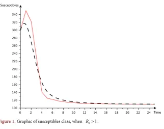
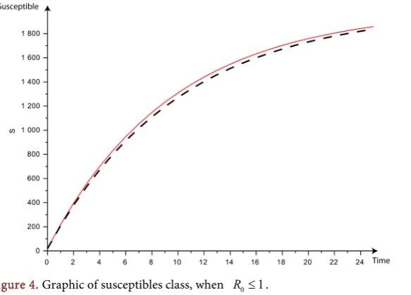
=0.021, we get R0=9.54 1> . It’ is important to notice that the software used is Scilab and the time is in term of weeks or months. In our graphic the red curve give the evolution of the class in the discrete model and the dashed ones give the evolution of the class in conti-nuous-time model.

Figure 1 present the evolution of the susceptibles population through the time, the dashed cuve represent the discrete model and the red one the continuous model when R0≤1.

Figure 2 give dynamic of the infected population along the time, the dashed cuve represent the discrete model and the red one the continuous model when

0 1

R ≤ _.

Figure 3 show the evolution of the recovered population through the time, the dashed cuve represent the discrete model and the red one the continuous model when R0≤1.

Figure 4 (Susceptibles population), Figure 5 (Infected population) and Figure 6

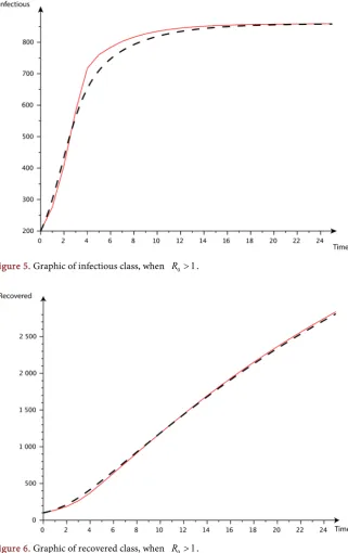
(Recovered population) represent the evolution through the time of the popula-tion when R0>1. The dashed cuves represent the discrete model and the red one the continuous model.

For all these cuves, we can see the convergence of the red cuves (the discrete model) and the dashed ones (the continuous model)

7. Conclusion

In this paper, we have studied a discrete SIR epidemic model with general

(13)

[image:13.595.241.525.73.273.2] [image:13.595.234.513.295.493.2]

DOI: 10.4236/am.2018.99070 1051 Applied Mathematics Figure 2. Graphic of infectious class, when R0≤1.

Figure 3. Graphic of recovered class, when R0≤1.

[image:13.595.236.528.517.726.2]

(14)

[image:14.595.213.535.73.584.2] [image:14.595.220.535.338.580.2]

DOI: 10.4236/am.2018.99070 1052 Applied Mathematics Figure 5. Graphic of infectious class, when R0>1.

Figure 6. Graphic of recovered class, when R0>1.

(15)

DOI: 10.4236/am.2018.99070 1053 Applied Mathematics dynamical properties for the step size

τ

=1 in the local and global stability of equilibra. These properties are nearly the same as the corresponding conti-nuous-time model (1). In our future work, it shall be important for us to study the same model, but with general positive step size

τ

and see how bifurcation can happen.

Acknowledgments

The authors want to thank the anonymous referee for his valuable comments on the paper.

Author’s Contribution

Aboudramane Guiro provide the subject, wrote the introduction and the con-clusion and verified some calculation. Dramane Ouédraogo conceived the study and computed the equilibria and their local stabilities. Harouna Ouédraogo rote mathematical formula, bring up the Lyapunov functional and did all the calculus with the other authors. All the authors read and approved the final manuscript.

Conflicts of Interest

The authors declare that they have no competing interests.

References

[1] Zhang, T. and Teng, Z. (2008) Global Behavior and Permanence of SIRS Epidemic Model with Time Delay. Nonlinear Analysis: Real World Applications, 9, 1409-1424. https://doi.org/10.1016/j.nonrwa.2007.03.010

[2] Cooke, K.L. (1979) Stability Analysis for a Vector Disease Model. Rocky Mountain Journal of Mathematics, 9, 31-42. https://doi.org/10.1216/RMJ-1979-9-1-31 [3] Guiro, A., Ouédraogo, D. and Ouédraogo, H. Global Stability for a Discrete SIR

Epidemic Model with Delay in the General Incidence Function. Submitted to Ad-vances in Difference Equations.

[4] Hethcote, H.W. (1976) Qualitative Analyses of Communicable Disease Models.

Mathematical Biosciences, 28, 335-356. https://doi.org/10.1016/0025-5564(76)90132-2

[5] Hethcote, H.W. (2000) The Mathematics of Infectious Diseases. SIAM Review, 42, 599-653. https://doi.org/10.1137/S0036144500371907

[6] Takeuchi, Y., Ma, W. and Beretta, E. (2000) Global Asymptotic Properties of a De-lay SIR Epidemic Model with Finite Incubation Times. Nonlinear Analysis, 42, 931-947. https://doi.org/10.1016/S0362-546X(99)00138-8

[7] Beretta, E., Hara, T., Ma, W. and Takeuchi, Y. (2001) Global Asymptotic Stability of an SIR Epidemic Model with Distributed Time Delay. Nonlinear Analysis, 47, 4107-4115. https://doi.org/10.1016/S0362-546X(01)00528-4

[8] Ma, W., Takeuchi, Y., Hara, T. and Beretta, E. (2002) Permanence of an SIR Epi-demic Model with Distributed Time Delays. Tohoku Mathematical Journal, 54, 581-591. https://doi.org/10.2748/tmj/1113247650

(16)

https://doi.org/10.1016/0025-5564(78)90006-8

[10] Xu, R. and Ma, Z. (2009) Global Stability of a SIR Epidemic Model with Nonlinear Incidence Rate and Time Delay. Nonlinear Analysis: Real World Applications, 10, 3175-3189. https://doi.org/10.1016/j.nonrwa.2008.10.013

[11] Connell McCluskey, C. (2010) Global Stability of an SIR Epidemic Model with De-lay and General Nonlinear Incidence. Mathematical Bioscience and Engineering

Volume 7, Number 4.

[12] Yoichi, E. and Yukihiko, N. (2010) Global Stability for a Class of Discrete SIR Epi-demic Models. Mathematical Biosciences and Engineering, Volume 7, Number 2. [13] Jang, S. and Elaydi, S.N. (2003) Difference Equations from Discretization of a

Con-tinuous Epidemic Model with Immigration of Infectives. Canadian Applied Ma-thematics Quarterly, 11, 93-105.

[14] Izzo, G. and Vecchio, A. (2007) A Discrete Time Version for Models of Population Dynamics in the Presence of an Infection. Journal of Computational and Applied Mathematics, 210, 210-221. https://doi.org/10.1016/j.cam.2006.10.065

[15] Izzo, G., Muroya, Y. and Vecchio, A. (2009) A General Discrete Time Model of Population Dynamics in the Presence of an Infection. Discrete Dynamics in Nature and Society, Art. ID: 143019, 15 p. https://doi.org/10.1155/2009/143019

[16] Sekiguchi, M. (2009) Permanence of Some Discrete Epidemic Models. International Journal of Biomathematics, 2, 443-461. https://doi.org/10.1142/S1793524509000807 [17] Hale, J. and Verduyn Lunel, S. (1993) Introduction to Functional Differential

Equa-tions, Springer-Verlag. https://doi.org/10.1007/978-1-4612-4342-7

[18] Van den Driesche, P. and Watmough, J. (2002) Reproduction Numbers and Subs-threshold Endemic Equilibria for the Compartmental Model of Disease Transmis-sion. Mathematical Biosciences, 180, 29-48.

[19] Lakshmikantham, V., Leela, S. and Martynyuk, A.A. (1989) Stability Analysis of Nonlinear Systems. Marcel Dekker, New York.