An analysis of the Romanian agriculture using quantitative methods

romania is the member of the European Union since January 2007. compared with the gDP per capita based on purchasing-power-parity (PPP) equal to 11 755 USD in 2009 (iMF estimation), romania is among the EU countries with a low level of economic development. considering the potential (area and population), romania is among the average countries in the EU. Under these conditions, agriculture is an important branch of the economy, creating 12.4% of gDP. About 30% of the country’s active population worked in this field during 2007. There was a down-ward trend of the share of the active population that works in agriculture before joining the EU from 37% in 2005 to 30% in the first year of the EU accession. This trend was mainly due to the external migration of the population and not of the national economic policies (Luca 2008).

Political changes that occurred in the early ‚90s re-sulted in major changes in the romanian agriculture. restitution of land owners who were expropriated in the period after the Second World War by the communist regime and the suppression of the

collec-tive associacollec-tive structures led to an excessive division of farmland. These are only two important factors that led to important changes in the organization of agricultural production in romania. Following the emergence of new legislation in this field immediately after the political changes of the late 80, there was significantly reduced the average area of holdings, reaching the level of 3.3 ha per 1 holding during 2007. This value ranks romania among the European countries with the highest level of fragmentation of arable land.

For the economy of a country where agriculture has a great potential, such as romania determined by natural conditions and the large number of persons who work in this sector, this activity is an important factor for social welfare. in literature, several studies have shown the relationship between demand and supply of labour from agriculture to the countries in transition. For example, grabowski and Sivan (1986) using a model of demand and supply studied the characteristics of agriculture sector in Japan, for the period 1885–1920 and Egypt for the period 1950–1974.

An analysis of the Romanian agriculture using

quantitative methods

Analýza rumunského zemědělství s využitím kvantitativních metod

Tudorel ANDREI

_{, Bogdan OANCEA}

_{, Marius PROFIROIU}

_{The Bucharest Academy of Economic Studies, Bucharest, Romania}

_{Nicolae Titulescu University, Bucharest, Romania}

Abstract: The paper presents a series of models used to identify the characteristics of the romanian agriculture in the 1960–2006 period of time. Using econometric methods we try to identify significant differences between agricultural pro-ductions obtained before and after the year of the revolution. Thus, following the dynamics of time series considered we identified two different time periods. The first is located before the 1989 revolution, and the second in the period that fol-lowed it. The two periods are different compared to the evolution of the considered indicators.

Key words:ADF test, regression models, agriculture evolution

Abstrakt:Článek přináší skupinu modelů, jež byly využity k identifikaci charakteristik rumunského zemědělství v období let 1960–2006. Snažili jsme se s využitím ekonometrických metod identifikovat významné rozdíly mezi zemědělskou pro-dukcí vytvořenou před rokem revoluce a po něm. na základě dynamických časových řad jsme tak identifikovali dvě časová období. První z nich je v období před revolucí 1989, druhé v období následujícím. Tato dvě období jsou výrazně odlišná, pokud jde o vývoj zkoumaných indikátorů.

The paper presents a series of models used to iden-tify the characteristics of the romanian agriculture in the 1960–2006 period. Using quantitative models, we try to identify the significant differences between agricultural productions obtained before and after the year of the revolution.

The paper is organized as follows. in the second part, we present the data series used in this paper for estimating econometric models. important fac-tors contributing to the development of modern agriculture were taken into consideration to define the data sets: the number of tractors, chemical fer-tilizer consumption and the farming population. To analyze the performance of agriculture, we analyzed the dynamics of the gross value added in agriculture and the average grain production per hectare.

next, we computed a number of descriptive sta-tistics trying to identify the characteristics in the data sets considered for analysis. Based on these results, we identified a number of distinct periods in the evolution of the romanian agriculture. We emphasized the existence of significant differences between the developments in agriculture before 1989 and after this year.

in the third and the fourth sections, we estimated the parameters for some econometric models used to analyze the dynamics of some variables from ag-riculture in the whole analyzed period and the two- sub periods identified by us. in the third part, we started with examining the stationarity of data series, and then we estimated the parameters of regression models used to identify the main factors that have contributed positively or negatively to the dynam-ics of labour productivity in agriculture during the whole period, and each sub-period separately. in the fourth section, we examined the evolution of the gross Value Added per 1 worker in agriculture. The

available data series allowed us to emphasize some characteristics of the romanian agriculture during 1961–2003. We used a series of econometric methods for analyzing the integration and co-integration of the data sets and to estimate the parameters of the regression models.

The econometric techniques used here are trying to answer a series of issues: the evolution on a long period of time of the labour productivity in agriculture (this is calculated as the added value per 1 farmer per year); contribution of the factors such as the technical endowment of the agricultural labour, expressed in terms of the average number of tractors per 100 ha, and the use of chemical fertilizers, the dynamics of labour productivity in the analyzed period and in some sub-periods; the evolution of the employ-ment share of agriculture in the total employemploy-ment in romania; identifying the important sub- periods in the development of agriculture.

DATA SERIES AND PRELIMINARY RESULTS

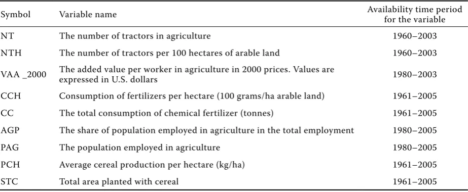
To conduct this study for romania, we used the data sets available in the latest yearbook published by the World Bank in 2008 (World Bank 2008). in the Table 1 below, there are shown the data series to be used, the periods for which they are available and the symbols for each series.

Based on the data sets for the variables defined in the above table, we calculated a series of statis-tical indicators and the data series are plotted in Figures 1, 3 and 4. The results allow the identifica-tion of sub-periods with different developments in the agriculture in romania. The average size of a farm is an important element to define the type of agriculture in the country. For this reason, in this

Table 1. Data series for romania published by the World Bank

Symbol Variable name Availability time period _{for the variable}

nT The number of tractors in agriculture 1960–2003

nTh The number of tractors per 100 hectares of arable land 1960–2003 VAA _2000 The added value per worker in agriculture in 2000 prices. Values are _{expressed in U.S. dollars} 1980–2003 cch consumption of fertilizers per hectare (100 grams/ha arable land) 1961–2005 cc The total consumption of chemical fertilizer (tonnes) 1961–2005 AgP The share of population employed in agriculture in the total employment 1980–2005

PAg The population employed in agriculture 1980–2005

Pch Average cereal production per hectare (kg/ha) 1961–2005

paper we present the size of agricultural holding for three years 1930, 1945 and 2007. The three values are shown in Figure 2.

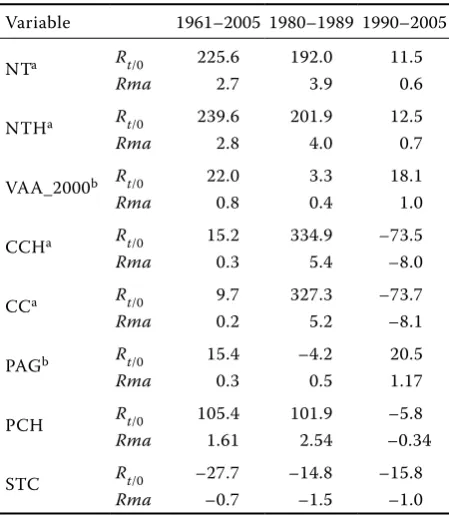
Thus, Table 2 shows the rates of changes for these variables (R_t/0= I_t/0 – 100 = (y_t/y₀ – 1)100), and annual average rate for each period considered

( ( )1 100 100)

0

t t y y

Rma ). The graphical representation

and descriptive statistics obtained allow the formula-tion of preliminary observaformula-tions on the identifica-tion of different sub-periods for the 1960–2005 time horizon, and also the characteristics of the variables related to the overall time horizon and each sub-period separately.

The first observation refers to the fact that for most variables, there is a noticeable upward trend since the beginning of the period until 1987. Then, for most vari-ables, there is observed a sharp decline since 1991.

The second observation emphasizes that during the first period, between 1961 and 1988, there is a continu-ously increase for the variable values that define the major issues relating to the modernization of agricul-ture: the number of tractors and fertilizer consump-tion. Thus, in 1961–1987 we are witnessing a growing number of tractors and consequently the number of tractors per 1 hectare of arable land. in contrast, in the period 1988–1991, there is a massive reduction in the number of tractors in agriculture. Thus, only in 1988, compared with the previous year, there was a decrease in the value of this variable to 10.2%. it is important to point out that the most significant decrease of this indicator was registered in 1990. This decrease was 12.4% compared with 1989. The total consumption of chemical fertilizers and that per 1 hectare increased during 1962–1984. During the next six years, there was a decrease, but not very sharp, of the consumption of chemical fertilizer in total and per hectare.

The year 1991 marked a sharp decrease of the two variables (see Figure 3). During the transition period, after 1991, the consumption of chemical fertilizers decreased at an average annual rate of 8%. in 2003, the average consumption of chemical fertilizers per hectare stood at the levels of the early sixties.

The third observation highlights that grain pro-duction per hectare has had an increasing trend until 1991. After this year, we found a high volatility of the grain yield per hectare. it should be noted that in 2000 romania recorded the lowest level of grain production per hectare in the past thirty years, the production being at the level of the late sixties. Another feature of this series is represented by large fluctuations from year to year since 1990. A moderate increase of this indicator was recorded for the period

–40 0 40 80 120 160 200

1960 1965 1970 1975 1980 1985 1990 1995 2000 2005 (%)

Figure 1. The evolution of the average an-nual grain production per 1 hectare in the period 1961–2006 compared with the pro-duction in 1961

Table 2.increasing/decreasing rate (R_t/0) and the yearly average rate (Rma) during time periods

Variable 1961–2005 1980–1989 1990–2005

nTa Rt/0 225.6 192.0 11.5

Rma 2.7 3.9 0.6

nTha Rt/0 239.6 201.9 12.5

Rma 2.8 4.0 0.7

VAA_2000b Rt/0 22.0 3.3 18.1

Rma 0.8 0.4 1.0

ccha Rt/0 15.2 334.9 –73.5

Rma 0.3 5.4 –8.0

cca Rt/0 9.7 327.3 –73.7

Rma 0.2 5.2 –8.1

PAgb Rt/0 15.4 –4.2 20.5

Rma 0.3 0.5 1.17

Pch Rt/0 105.4 101.9 –5.8

Rma 1.61 2.54 –0.34

STc Rt/0 –27.7 –14.8 –15.8

Rma –0.7 –1.5 –1.0

1980–1990, but given that the fluctuations from year to year were very low.

The fourth observation is that during 1980–1990, the population employed in agriculture and its share in the total employment in the economy stayed rela-tively constant. Massive restructuring of the industry in the early nineties led to a significant increase in two indicators. A significant reduction of the two indicators has been recorded starting with 2000.

This trend was not due to the economic reforms but rather to the massive population migration to Western countries, mainly to italy and Spain.

in the fifth place, there has to be reported the role of the average surface size of farms on agricultural production. As in some other central and Eastern European countries (Sklenička et al. 2009), the land ownership fragmentation when the non-contiguous plots of individual owners are scattered around the

73.7

86.3

49.8

15.9 _14.6

12.6 10.4

0

37.6

0 30 60 90

1930 1945 2007

(%)

under 10 ha 10-100 ha over 100 ha

Figure 2. Farms area distribution in 1930, 1945 and 2007

0 400 800 1200 1600 2000

1965 1970 1975 1980 1985 1990 1995 2000 CCH

CH 0

400000 800000 1200000 1600000 2000000

1965 1970 1975 1980 1985 1990 1995 2000 CC

40000 60000 80000 100000 120000 140000 160000 180000 200000

1965 1970 1975 1980 1985 1990 1995 2000 NT

40 60 80 100 120 140 160 180 200

1965 1970 1975 1980 1985 1990 1995 2000 NTH

area of one or more cadastres has a negative role in the agriculture development. We noticed as a nega-tive consequence of measures taken after 1990 the continuous reducing of the agricultural areas for grain cultivation. According to (Luca 2009), in romania, there are two different agriculture. The first includes small holdings of over 2.6 million households which have an area of less than 1 ha. They provide the farm households own consumption and the production is not intended for the consumer market. in the sec-ond category, there are included large farms as total over 100 hectares each. This category includes over 9600 exploitations. Figure 2 shows the distribution of agricultural areas by the type of exploitation in 1930, 1945 and 2007. As a result of the legislative actions taken in the last time, we find a reduction in the share of small farms.

After the Second World War, small farms were predominant. As a result of the forced collectivization made in romania in 1950–1960, there was a consoli-dation of agricultural areas and a reduction in the share of the small farms. The fall of the communism marked the beginning of the period of the land resti-tution to the owners and the reducing of the size of agricultural holdings. in 2007, approximately 50% of the farmland have an area smaller than 10 ha. There must be noticed the high share of agricultural area

owned by large agricultural holdings in 2007. Thus, the farms larger than 100 ha represent 37.6% of the romania’s agricultural area.

THE ANALYSIS MODELS

Using the ADF test, we will determine the order of integration of the variables defined in Table 1. To apply this test, we considered the methodology for implementing the ADF test described in Baltagi (2008). in the case of the ADF test, we estimated three models to determine if the process is stationary:

M₁: t

p

j j t j t

t Y Y

Y I I ' H

'

¦

1

1 (1)

M₂: t

p

j j t j t

t c Y Y Y I I ' H

'

¦

1

1 (2)

M₃: t

p

j j t j t

t c at Y Y Y I I ' H

'

¦

1

1 (3)

The two hypotheses of the test are defined as fol-lows:

h₀: I 0œ series is non-stationary and has a unit root

h₀: I0œ _{series is stationary and has no unit root} 4000

4400 4800 5200 5600 6000 6400

80 82 84 86 88 90 92 94 96 98 00 02 VAG

.24 .28 .32 .36 .40 .44

80 82 84 86 88 90 92 94 96 98 00 02 AGP

2800 3200 3600 4000 4400 4800 5200

80 82 84 86 88 90 92 94 96 98 00 02 POA

The null hypothesis is accepted if the statistics of the coefficient Φ based on the data series is greater than the critical value determined by the model type, the size of the data series and the significance level.

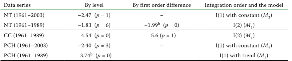
The results for the three variables after applying the above procedure for the stationarity analysis are presented in Table 3.

The results allow the formulation of the following conclusions about the evolution of the long-term data series on important variables quantifying important fac-tors in this sector (evolution of the number of tracfac-tors and chemical fertilizer consumption), but also of the results in this area of activity (production of cereals).

The nT is a non-stationary variable, with a dif-ferent integration order in certain sub-periods of time. Thus, for the time period 1961–1989, it is an integrated process of second order (i (2)), while for the whole time horizon; it is a process i (1). in the latter case, the model is presented as a model M2. The variable ΔNT_t allows the following representa-tion for 1961–1989 (Table 4)

nT, Pch and cc variables have different character-istics related to their evolution throughout the entire time horizon considered. Moreover, for each of the

three variables, there are different representations for the two time horizons (1961–1989, 1990–2005 respectively).

The grain production per hectare is non-station-ary for the 1961–2003 time frames, but things are different in the two sub-periods of time identified. Tables 5 and 6 show the features of the M2 and M3 models estimated for grain production per hectare based on the data from 1961 to 1989 period, and respectively from 1961 to 2003.

ANALYSIS MODELS FOR GROSS VALUE ADDED

The regression model proposed here attempts to analyze the dynamics of gross value added per 1 worker in agriculture depending on a number of important factors such as the employment share of agriculture, the consumption of fertilizers per hectare, the average number of tractors on 100 hectares of arable land and the changes that took place in the romanian agricul-ture since 1990. The model estimation is performed in three different situations.

Case 1. The first is the case where the data series for the whole analyzed period are used for the pa-rameters estimations, without taking into account the exceptional evolutions of various sub- periods in agriculture. in this case, the regression model is defined by the relationship below:

t t t

t

t NTH AGP CCH

VAA_2000) D D log( )D log( )D log( )H

log( _{0 1 2 3}

t t t t

t NTH AGP CCH

VAA_2000) D D log( )D log( )D log( )H

log( _{0 1 2 3 (4)}

Table 3. ADF test for three variables

Data series By level By first order difference integration order and the model

nT (1961–2003) –2.47 (p = 1) – i(1) with constant (M₂)

nT (1961–1989) –1.83 (p = 6) –1.99b _{(p = 0) i(2) (M} 1)

cc (1961–1989) –4.54 (p = 0) –5.6 (p = 1) i(2) (M₁)

Pch (1961–2003) –2.40 (p = 3) – i(1) with constant (M₂)

Pch (1961–1989) –3.74b _{(p = 0) – i(1) with trend (M}

3) The critical values of the test for a siginficance level of 1%, 5%, 10% are –4.67, –3.73, –3.31

a_{significant for 1%;} b_{significant for 5%;} c_{significant for 10%}

Table 4. M₂ model for nT variable for 1961–1989 Variable coefficient Std. Error indices nT(-1) –0.066400 0.036349

R2 _{= 0.70} DW = 2.12 AIC = 20.12 F = 4.7 D(nT(-1)) 0.833395 0.193557

D(nT(-5)) 0.708566 0.288550 D(nT(-6)) –0.969419 0.307174

c 11 732.44 6 057.742

Table 5. M₃ model for Pch variable for 1961–1989 Variable coefficient Std. Error indices Pch(-1) –0.762332 0.203876 R2 _{= 0.40}

DW = 1.97 AIC = 13.93 F = 7.17

c 1 244.940 319.2775

@TrEnD(1961) 48.08490 14.90713

Table 6. M₂ model for Pch variable for 1961–2003 Variable coefficient Std. Error indices Pch(-1) –0.269642 0.112431 R2 _{= 0.50}

DW = 2.07 AIC = 14.60 F = 18.9 D(Pch(-1)) –0.530769 0.125106

Case 2. in the second case, we take into account that, in 1990 and 1991, due to the weather conditions and psychological reasons that agricultural establishments have benefited from, the gross value added of this sector was much higher than in the remaining years of the analyzed period. in this case, the above model introduces a dummy variable defined as:

¯ ® ­

1991 , 1990 ,

0

2003 ..., , 1992 , 1989 ..., , 1980 ,

1 1

t t

VD (5)

Under these conditions, the regression model is writ-ten in the form below:

t t t

t

t NTH AGP CCH VD

VAA_2000) D D log( )D log( )D log( )D 1 H

log( 0 1 2 3 4

t t t t

t NTH AGP CCH VD

VAA_2000) D D log( )D log( )D log( )D 1 H

log( 0 1 2 3 4 (6)

Case 3. in the third situation, we studied the potential differences between the 1980–1989 and 1992–2003 periods. in addition, in this case, we considered the comments that were made to define the model in the second case. in this model, we introduced in addition a dummy variable VD that is defined as follows:

¯ ® ­

2003 ..., , 1992 ,

0

1991 ...., , 1980 ,1

t t

VD (7)

This variable is inserted to determine whether the characteristics referred to the two sub-periods are different. Under these conditions, we obtain the regression model below:

t t t

t t

t NTH AGP CCH VD VD VAA_2000) D₀D₁log( )D₂log( )D₃log( )D₄ 1 D₅ H

log(

t t t t

t

t NTH AGP CCH VD VD VAA_2000) D₀D₁log( )D₂log( )D₃log( )D₄ 1 D₅ H

log( ₍₈₎

The parameters estimations for the last three models were made with various combinations of variables

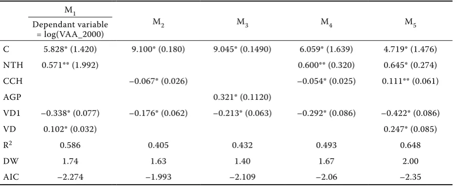
that were described in Table 1. The explained variable of the regression model is the logarithm of the gross value added per 1 worker expressed in the year 2000 prices (log (VAA_2000), and the parameter estimation was done by the least squares method. The results are presented in Table 7.

These results allow us to formulate the follow-ing comments on the factors contributfollow-ing to the dynamics of labour productivity in agriculture: All models highlight the negative effect played by the consumption of fertilizers per 1 hectare of arable land on labour productivity in agriculture in the period 1989–2006. The results show that this factor played a positive role on the evolution of the gross value added in agriculture in the period 1961–1988. The evolution of factors considered with regard to the gVA is different in the two sub-periods consid-ered (1961–1988 and 1989–2006). Mechanization of agriculture, mainly by increasing the number of tractors, has contributed significantly to the agricul-tural development throughout the analyzed period. in this case, the positive impact of this factor is more important in the period 1961–1987.

CONCLUSIONS

For the time horizon considered in our analysis, agriculture in romania has seen various developments in the various sub-periods of time. Thus, following the dynamics of the time series considered here, we identified two different time periods. The first is lo-cated before 1989, and the second in the period that followed it. The two periods are different compared to the evolution of the considered indicators.

Table 7. regression models for the analysis of VAA_2000 M₁

M₂ M₃ M₄ M₅

Dependant variable = log(VAA_2000)

c 5.828* (1.420) 9.100* (0.180) 9.045* (0.1490) 6.059* (1.639) 4.719* (1.476)

nTh 0.571** (1.992) 0.600** (0.320) 0.645* (0.274)

cch –0.067* (0.026) –0.054* (0.025) 0.111** (0.061)

AgP 0.321* (0.1120)

VD1 –0.338* (0.077) –0.176* (0.062) –0.213* (0.063) –0.292* (0.086) –0.422* (0.086)

VD 0.102* (0.032) 0.247* (0.085)

r2 _{0.586 0.405 0.432 0.493 0.648}

DW 1.74 1.63 1.40 1.67 2.00

Aic –2.274 –1.993 –2.109 –2.06 –2.35

Significant changes recorded in the agriculture in romania after 1990 were mainly represented by: land restitution to the dispossessed owners after the second world war; the change of the regime of agri-cultural land circulation; change of the agriagri-cultural units organization; the lack of interest from the state to conserve irrigation systems; eliminating customs barriers for agricultural products from abroad and the emergence of competitors, etc. it should be noted that after the political changes in late 1989, the two main laws that were adopted in agriculture are mainly aimed at creating the legal framework for the land restitution and were less oriented at the support implementing a coherent agricultural policy.

The first consequence of these developments was reducing of the average area of holdings. in late 2007, romania with the average of 3.3 ha per 1 holding is among the countries with the highest level of frag-mentation of arable land.

The second negative consequence of the measures taken after 1990 in the agriculture has been represented by the continuous reduction of the agricultural areas for grain cultivation. During 1990–2005, the agricultural area cultivated with cereals decreased by over 15% in the average annual rate of 1%. Moreover, during this period, large agricultural areas have remained uncul-tivated. Small productions per hectare, high costs and the lack of domestic markets to exploit the primary production of cereals are among the main factors de-termining the resting of large agricultural areas.

The third major negative consequence of the eco-nomic policy in agriculture was represented by the continuous increase in the share of the population employed in agriculture, together with economic policies that led toward a massive deindustrialization of romania. Agriculture in romania is currently an important part of the employed population of the country. it has grown massively in the ensuing po-litical changes of 1989, mainly due to the country’s industrialization process (Andrei et al. 2007). in 1990,

there worked in agriculture about 28.5% of the em-ployed population, and this share increased to 43.5% in 2001. Yet the importance decreases were recorded since 2002, so it was at 30% in 2008. This decreasing trend was not due to the reforms in the economy generally and especially to those in agriculture, but due to the large number of people who left to work abroad since 2002.

Acknowledgements

The work related to this paper was supported by the cncSiS–UEFiScSU project Pnii – iDEi iD_1814.

REFERENCES

Andrei T., iacob A., Vlad L. (2007): Tendencies in the ro-mania’s regional economic development during the pe-riod 1991–2004. Economic computation and Economic cybernetics Studies and research, 41: 107–120. Baltagi B. (2008), Econometrics. 4th _{ed. Springer, Berlin.} grabowski r., Sivan D. (1986): The supply of labor in

agriculture and food prices: The cases of Japan and Egypt, 14: 441–447.

Luca L. (2009): A country and two agricultures – romania and the reform the cAP of the EU (o tara si doua agri-culturi-romania si reforma Politicii Agricole comune a UE).Policy Memo nr. 4, centrul roman de Politici Europene, Fundatia Soros-romania.

Sklenicka P., hladík J., Střeleček F., Kottová B., Lososová J., Číhal L., Šálek M. (2009): historical, environmental and socio-economic driving forces on land ownership fragmentation, the land consolidation effect and the project costs. Agricultural Economics – czech, 55: 571–582.

World Bank (2008). Agriculture and Achieving the Mil-lennium Development goals. World Bank, Agricul-ture and rural Development Department, report no. 32729-gLB.

Arrived on 9th _{May 2010}

Contact address:

Tudorel Andrei, Marius Profiroiu, The Bucharest Academy of Economic Studies, 6, romana Square, District 1, 010374 Bucharest, postal office 22, romania