Influence of rainfall data on the uncertainty of flood simulation

Influence of Rainfall Data on the Uncertainty

of Flood Simulation

Andrzej WALEGA

1

_{and Leszek KSIAZEK}

2

1_{Department of Sanitary Engineering and Water Management and} 2_{Department of Water}

Management and Geotechnics, University of Agriculture in Krakow, Krakow, Poland

Abstract

Walega A., Ksiazek L. (2016): Influence of rainfall data on the uncertainty of flood simulation. Soil & Water Res., 11: 277−284.

The aim of this paper was to determine the influence of factors related to rainfall data on the uncertainty flood simulation. The calculations were based on a synthetic unit hydrograph NRCS-UH. Simulation uncertainty was determined by means of GLUE method. The calculations showed that in the case of a catchment with limited meteorological data, it is better to use rainfall data from a single station located within the catchment, than to take into account the data from higher number of stations, but located outside the catchment area. The pa-rameters of the NRCS-UH model (curve number and initial abstraction) were found to be less variable when the input contained rainfall data from a single rainfall station. It was also manifested by a lower uncertainty of the simulation results for the variant with one rainfall station, as compared to the variant based on the use of averaged rainfall in the catchment.

Keywords: calibration; GLUE method; model quality; rainfall-runoff model

Modelling of hydrological processes requires knowl-edge on local conditions related to the water cycle (Kovář et al. 2015). To accurately estimate floods with hydrological models, the model parameters and the initial state variables must be known. Good estimations of parameters and initial state variables are required to enable the models to make accurate estimations (Lü et al. 2013). According to Butts et al. (2004), the key factors determining the simulation accuracy involve input parameters and the hydrolo-gist’s knowledge of the model structure. Important factor, affecting the model outcomes, is the quality of information constituting the model input, mainly the precipitation data. Bormann (2006) indicated that high quality simulation results require high quality input data, but not necessarily always highly resolved data. The studies performed by Bárdossy and Das (2008) showed that the number and spatial distribu-tion of the rain gauges affect the simuladistribu-tion results. Anctil et al. (2006) showed that model performance was rapidly reduced when the mean area rainfall

was computed using a number of rain gauges lower than a certain number. Spatial distribution and the accuracy of the rainfall input to a rainfall-runoff model considerably influence the volume of storm runoff, peak runoff, and time-to-peak. Errors in storm-runoff estimation were directly related to spatial data distribution and the representation of spatial conditions across a catchment.

A variety of methods has been developed to deal with parameter uncertainty and modelling uncertain-ty. Among these methods, the generalized likelihood uncertainty estimation (GLUE) method, developed by Beven and Binley (1992), and the formal Bayesian method using Metropolis-Hastings (MH) algorithm, a Markov Chain Monte Carlo (MCMC) methodol-ogy, are extensively used (Bates & Campbell 2001; Blasone et al. 2008). Most studies were carried out in the catchments where detailed hydrological and meteorological data were available. However, there are situations when hydrological calculations are necessary, e.g. for the purpose of flood protection, but the catchments are poorly metered (limited num-ber of gauges and rainfall stations). Then, the use of hydrological models is particularly difficult, as the calibration process is based on a limited amount of data. This can increase the uncertainty of simulation results. During major social and economic changes oc-curring in the 1980s and 1990s, the number of gauges and rainfall stations in Poland was seriously limited. As a result, only large catchments (with an area of over several thousand km2_{) have a dense network of}

meteorological and hydrological stations. Smaller catchments often feature just one or two gauges and rainfall stations, and sometimes this infrastructure is completely absent. Implementation of flood pro-tection plans requires also hydrological analyses to be conducted, often with the use of hydrological models, in the catchments with under-developed measurement network. Moreover, designers usu-ally base their calculations on basic hydrological models, mostly those of lumped parameters, due to their simplicity and ease of obtaining and setting the parameters. Therefore, a question arises whether the uncertainty of hydrological calculation obtained for catchments with poor hydro-meteorological data shall disqualify the applied hydrological models.

Thus, the aim of this paper was to determine the influence of factors related to rainfall input data quality on the uncertainty of flood parameters ob-tained from a simulation. The uncertainty analysis concerned only a direct runoff during a flood, as it was the main component of the total runoff in the investigated catchment, and the applied methodolo-gies required only this concrete runoff component for further hydraulic modelling of water transformation in the river beds.

Characteristics of the Stobnica River and the

catchment area. The study included an upland river

Stobnica – right-bank tributary of the Wislok,

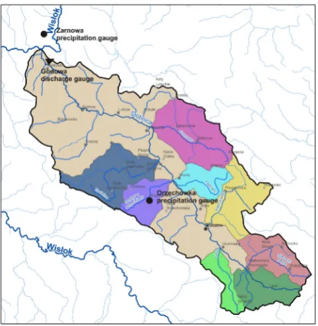
situ-ated in the south-eastern part of Poland (Figure 1). The catchment is located in the temperate climate zone. Its area is 335.84 km2_{, and the length of the}

main watercourse is 47.319 km. Mean catchment slope is 0.78%. The catchment soils are mainly of poor and medium permeability. Most of its area is covered by arable land and forests.

The average annual rainfall in the Stobnica catch-ment for the years 1971–2000 was about 650 mm, and the average number of days with thunderstorms per year was 28–30. There is a river gauge on the Stobnica River, located in Godowa at 2.773 km. Only two rainfall stations are currently located within the catchment or in its vicinity: Orzechowka, in the central part of the catchment, and Zarnowa (outside the catchment boundaries, but covering the Stobnica estuary area).

MATERIAL AND METHODS

[image:2.595.304.534.485.721.2]

Daily precipitation was measured at the rainfall stations in Zarnowa and Orzechowka, flow hydro-graphs were obtained for the river gauge in Godowa as recorded in the years 1997–2010. The data were obtained from the Institute of Meteorology and Water Management, National Research Institute in Warsaw. The Institute’s archives contained only the data on flow and rainfall for a daily time step.

In total, sixteen greatest rainfall-runoff events per year were selected for the analysis.

The analyses were carried out as follows: first, the parameters of the hydrological model were calibrated, taking into account the rainfall recorded at one rainfall station Orzechowka, located in the central part of the catchment. Then, the model parameters were cali-brated, taking into account averaged catchment rainfall recorded at two rainfall stations. The averaged catch-ment rainfall was determined using Thiessen method. All calculations were performed using HEC-HMS 3.4 software (USACE 2008). The calibration involved curve number (CN) parameter and initial abstraction (Ia). The univariate gradient search method of the HMS optimization manager was applied in the automated model calibration to optimize the set of initial model parameters within the limits obtained by manual cali-bration (Cunderlik & Simonovic 2004). The model quality was determined by using the following indices: – efficiency coefficient E (Nash & Sutcliffe 1970):

(1)

– percentage error in peak flow rate PEP (%):

(2)

– percentage error in wave volume PEV (%):

(3)

– percentage weight root mean square error PWRMSE (%):

(4)

where:

N – number of ordinates of the hydrograph

i – index varying from 1 to N

Q_o(t) – ith _{ordinate of the observed hydrograph}

Q_s(t) – ith _{ordinate of the simulated hydrograph}

Q_m – mean of the ordinates of the observed hydrograph

Q_s,max – simulated peak discharge

Q_o,max – observed peak discharge

V_s – simulated volume of hydrograph

V_o – observed volume of hydrograph

We adopted the criterion proposed by Moriasi et al. (2007), assuming that for E values above 75% the model-based reality description was very good, for E in the range of 65–75% it was good, and for E = 50–64% satisfactory. Initial values of CN parameter were determined based on observed rainfall-runoff episodes. Initial value of Ia parameter was assumed 0.20∙S, when S is the maximum potential retention according to USDA (1986).

Further steps involved uncertainty analysis of the simulation results based on generalized likelihood uncertainty estimation (GLUE) method. The procedure is based on running a large number of Monte Carlo (MC) model simulations with different parameter sets, sampled from proposed (prior) distributions, and infer-ring the outputs and parameter (posterior) distributions based on the set of simulations showing the closest fit to the observations (obtained from parameter sets defined as “behavioural”) (Blasone 2007). A priori distribution of the model parameters was determined based on the observed floods. Monte Carlo simulations were run for the variant with a single rainfall station and for the variant with averaged rainfall from two rainfall stations. Here, the performance of each model was evaluated by multiple performance or likelihood measures. In most applications of GLUE, parameter sampling is carried out using non-informative uniform sampling without prior knowledge of individual param-eter distribution other than a feasible range of values (Chen et al. 2013). In this study, the Nash-Sutcliffe efficiency (Nash & Sutcliffe 1970) was chosen for the likelihood function as in many other studies. The likelihood function was calculated based on Eq. (1).

In order to provide a quantitative evaluation of the difference between the results of the different rainfall data, the following uncertainties were calculated:

Average relative length (ARIL) is proposed by Jin et al. (2010) as follows:

(5)

Average asymmetry degree (AAD) of the predic-tion bounds (Xiong et al. 2009) with respect to the corresponding observed discharge is simulated:

(6)

Average deviation amplitude (ADA) is used by Xiong et al. (2009) as follows:

(7)

E =

[

1 − ∑ (Qo(t) − Qs(t))2

]

∑ (i=N Qo(t) − Qm)2

i=1 i=N

i=1

PEP =

(

1 − Qs,max

)

_{× 100} Qo,max

PEV =

(

1 − Vs

)

_{× 100} Vo

PWRMSE = 100 ×

√

∑ (Qo(t) − Qs(t))2 ×

Q_o(t) − Q_m

N N

t=1 2Qm

Q_m = 1 − ∑ Q_o(t)

N N t=1

ADD = 1

∑

|

Limitu,t − Qobst,t _{− 0.5}

|

n Limitu,t −Limitl,t

n i=1

ARIL = 1

∑

Limitu,t − Limitl,t n Qobst,t

n i=1

where:

Limit_l,t, Limit_u,t – lower and upper boundary values of 95% confidence intervals

Q_obs,t – observed flow (for all n ordinates of the observed hydrograph)

n – number of time steps

At the last stage of the calculations, the model was verified using independent materials, based on the observed flood that occurred in June 1999.

For the Stobnica catchment, the total runoff hydro-graph was calculated based on rainfall-runoff model developed by the Natural Resources Conservation Service (NRCS) (Bedient et al. 2013). An extremely important parameter, describing a catchment response to rainfall, is the lag time. As in the case of the Stobnica catchment, this parameter was determined by means of a direct method in each sub-catchment, its initial value was determined using the following formula:

(8)

where:

T_lag – lag time (h)

L – catchment length (km) CN – curve number

J – catchment slope (%)

These rainfall events were the basis for the cal-culation of the effective rainfall, representing the

direct runoff. The effective rainfall was calculated by NRCS-CN method where CN initial values were determined based on land use, soil conditions, and hydrological conditions in each sub-catchment.

RESULTS AND DISCUSSION

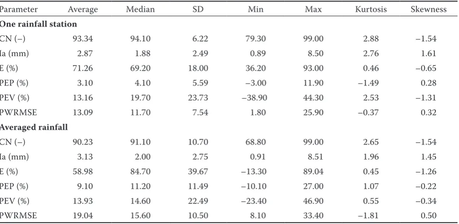
Calibration of the model parameters. Table 1

shows the results of the calibration of NRCS-UH model parameters, depending on the variant for deter-mining the rainfall in all the observed rainfall-runoff episodes. The analyses demonstrated significantly higher scores achieved by the model calibrated with the input data coming from a single rainfall station Orzechowka. This was evidenced by higher values of E coefficient, and lower values of PEP, PEV, and PWRMSE in the model using the data from a sin-gle rainfall station, as compared to the model with spatially averaged rainfall data used as the input information. The values of CN and Ia parameters were also different, depending on the quality of the rainfall data used. Regardless of the quality of the rainfall data, the values of CN and Ia parameters were characterized by asymmetric distribution, as evidenced by the kurtosis and skewness values.

According to the classification of Moriasi et al. (2007), average E coefficient values for a model based on a single rainfall station allowed for classifying this model as a good one. In 44% of the simulations, the

T_lag = (3.28 × L × 1000)0.8 ×

(

1000 − 9

)

0.7

[image:4.595.65.533.503.731.2]

1900 √J CN

Table 1. The results of synthetic unit hydrograph NRCS-UH model calibration for the observed rainfall-runoff episodes

Parameter Average Median SD Min Max Kurtosis Skewness

One rainfall station

CN (–) 93.34 94.10 6.22 79.30 99.00 2.88 –1.54

Ia (mm) 2.87 1.88 2.49 0.89 8.50 2.76 1.61

E (%) 71.26 69.20 18.00 36.20 93.00 0.46 –0.65

PEP (%) 3.10 4.10 5.59 –3.00 11.90 –1.49 0.28

PEV (%) 13.16 19.70 23.73 –38.90 44.30 2.53 –1.31

PWRMSE 13.09 11.70 7.54 1.80 25.90 –0.37 0.32

Averaged rainfall

CN (–) 90.23 91.10 10.70 68.80 99.00 2.65 –1.54

Ia (mm) 3.13 2.00 2.75 0.91 8.51 1.96 1.45

E (%) 58.98 84.70 39.67 –13.30 89.04 0.45 –1.26

PEP (%) 9.10 11.20 11.49 –10.10 27.00 1.07 –0.22

PEV (%) 13.93 14.60 22.49 –23.40 46.90 0.55 –0.34

PWRMSE 19.04 15.60 10.50 8.10 33.40 –1.81 0.50

quality of the model based on a single rainfall station was found to be very good, in 22% of the simulations it was good, in 22% satisfactory, and in 16% inadequate. When catchment-averaged rainfall was used as the input data, the quality of the simulation markedly deteriorated, and an average value of E coefficient indicated the outcomes calculated with NRCS-UH model as satisfactory. In 57% of the simulations, the quality of the model based on averaged rainfall was assessed as very good, in 15% of cases it was found to be satisfactory, and in 28% inadequate.

Uncertainty analysis. The data set obtained as a

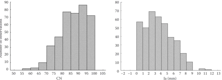
result of Monte Carlo simulation was used to assess the model uncertainty. Figures 2 and 3 present histograms with an empirical distribution of the NRCS-UH model parameters depending on the quality of the rainfall data.

Asymmetric distribution was achieved for each of the analyzed parameters. In the case of the simula-tion with a single rainfall stasimula-tion, the distribusimula-tions were unimodal. The highest count of values was noticed within the range of 90–98 for the CN pa-rameter, and from 1.0 to 4.0 mm for Ia parameter. The histogram of the CN parameter for the model including averaged rainfall was unimodal, and the largest number of observations was found for the CN range 80–99. In the case of Ia parameter, the distribution was bimodal, and the largest number of this parameter occurrences was recorded within the range of 0.1–5.0 mm.

[image:5.595.70.533.95.276.2]

The next stage of the analysis involved a selection of the model parameters yielding the best simula-tion quality and describing them using a posterior Figure 2. Histograms of curve number (CN) and initial abstraction (Ia) parameters for the simulations based on the rainfall data from a single station

Figure 3. Histograms of curve number (CN) and initial abstraction (Ia) parameters for the simulations based on the averaged rainfall data

N

umb

er of ob

ser

va

tions

CN Ia (mm)

72 74 76 78 80 82 84 86 88 90 92 94 96 98 100 102 70

60

50

40

30

20

10

0

90 80 70 60 50 40 30 20 10 0

−2 −1 0 1 2 3 4 5 6 7 8 9 10 11 12 13

N

umb

er of ob

ser

va

tions

CN Ia (mm)

50 55 60 65 70 75 80 85 90 95 100 105 80

70

60

50

40

30

20

10

0 90

80 70 60 50 40 30 20 10 0

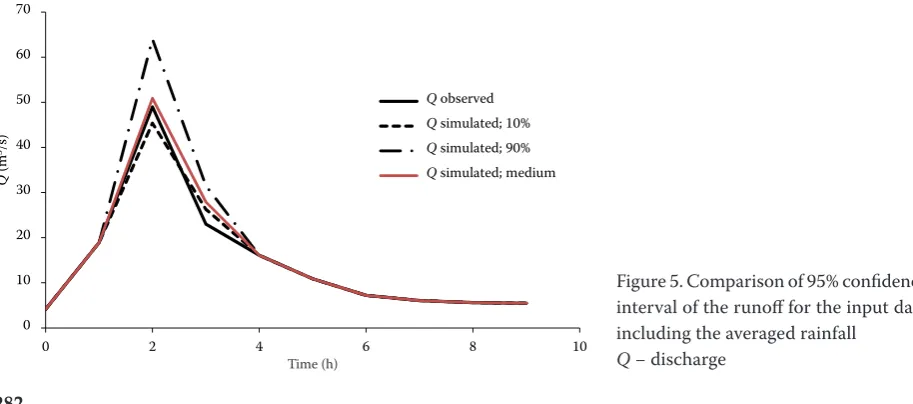
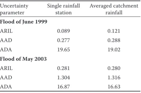
[image:5.595.66.529.560.727.2]

distribution. A selection criterion was the threshold value of likelihood function, defined by the Eq. (1) and exceeding 65% which, as previously mentioned, denoted good and very good models. The simula-tions, in which the values of E were below 65%, were excluded from further analysis. Figure 4 shows the simulation results with the uncertainty area for the rainfall data from a single rainfall station, and Fig-ure 5 depicts the variant in which the model input included the averaged rainfall. Table 2 presents the calculated uncertainty results.

The presented calculations seem to indicate that the resulting hydrograph correctly described the investi-gated flood. The simulations, in which the input data included the rainfall from a single station, showed that the hydrograph was located in the middle of 95% confidence interval, within the ascending part, and the beginning of the regression part. In the remaining part it was outside the lower limit of the confidence interval. In the case of the simulation based on the averaged catchment rainfall, the resulting hydrograph was located

[image:6.595.66.391.91.268.2]

within the lower limit of the confidence interval in the ascending part and the beginning of the regression part, and in the remaining phase the hydrograph was beyond the lower limit of the confidence interval. In order to provide a quantitative evaluation of the difference among the results of the simulation, ARIL, AAD and ADA were calculated (Table 2). An AAD value lower than 0.5 indicated that, on average, the observed discharge was within the uncertainty bands, whereas the higher the AAD value, the more asymmetrical the uncertainty bands were around the observed water levels (Xiong et al. 2009). For example, in Eq. (6) replace the h, we get |h – 0.5| for each time step. If the prediction bounds were completely symmetrical around Q, which is the ideal case, such that Q was equal to the middle point value of prediction bounds, h = 0. Hence, the closer the bounds values are to their respective Q values, the closer will be the corresponding h values to 0.5 and the respective expression |h – 0.5| is also close to zero, indicating almost perfect symmetry of the bounds about the discharge hydrograph.

Figure 5. Comparison of 95% confidence interval of the runoff for the input data including the averaged rainfall

Q − discharge

0 10 20 30 40 50 60 70

0 1 2 3 4 5 6 7 8 9 10

Q

(m

3/s)

t (h)

Q observed

Q simulated; 10%

Q simulated; 90%

Q simulated; median

Time (h)

0 10 20 30 40 50 60 70

0 2 4 6 8 10

Q

(m

3/s)

t (h)

Q observed

Q simulated; 10%

Q simulated; 90%

Q simulated; medium

[image:6.595.67.524.573.775.2]

Time (h)

Figure 4. Comparison of 95% confidence interval of the runoff for the input including data from a single rainfall station

When hydrological calculations are required in the catchments equipped with a limited number of rainfall stations, the simulations are more accurate if the data from a lower number of stations are used, preferably those located within the catchment and/or close to its borders. In the case of June 1999 flood, it was demonstrated by slightly higher ARIL and AAD values in the variant with averaged rainfall, as compared with the variant accounting for rainfall time series from only one station. However, it can be concluded that, regardless of the quality of the rainfall data, the model uncertainty was at a similar level, as the resulting hydrograph was within 95% confidence interval. The model accounting for only one rainfall station was characterized by a slightly higher deviation amplitude. On the other hand, a greater uncertainty of the simulation results was obtained for the flood of May 2003. Compared to the flood of 1999, ARIL and AAD values were higher, and an opposite situation was perceived for ADA. The analysis of the second flood showed an asym-metric position of the resulting hydrograph and the confidence limits, regardless of the quality of input rainfall data (AAD value above 0.5). A significant part of the hydrograph for the second flood was located outside the confidence limits. However, it was noticed that the uncertainty was slightly lower in the simulations of the 2003 flood for the vari-ant based on the rainfall data from a single station. This was due to the fact that one of the rainfall sta-tions (Orzechowka) was located within the catch-ment area, and the other (Zarnowa) was outside the catchment. Supplying the model with the averaged rainfall from two stations increased the uncertainty

of simulation results, because the rainfall recorded at Zarnowa station only slightly affected the flood wave formation in the Stobnica River. Effects of the rainfall recorded at this station were limited mainly to the estuary area, while an essential volume of the runoff was formed in the upper and central part of the catchment.

CONCLUSION

The article discussed the effects of the rainfall data quality on the uncertainty of flood simulation using the NRCS-UH model. The study was conducted in the catchment area of the Stobnica River in south-eastern Poland. It is a catchment where limited hy-drological and meteorological data are available, which undoubtedly makes the practical application of hydrological models difficult. We analyzed the rainfall data obtained from a single rainfall station or averaged for two stations and used as the model input. The calculations showed that in the case of a catchment with limited meteorological data, it is better to use rainfall data from a single station located within the catchment, than take into account the data from a higher number of stations, but located outside the catchment area. Based on the model uncertainty calculations, carried out as per GLUE method, the parameters of NRCS-UH model (CN and Ia) were found to be less variable when the input consisted of the rainfall data from a single rainfall station. It was also manifested by lower uncertainty of the simulation results for the variant with one rainfall station, as compared with the variant using averaged catchment rainfall.

Acknowledgements. The authors gratefully acknowledge

the Institute of Meteorology and Water Management, Nati-onal Research Institute in Warsaw, Poland, for providing the hydro-meteorological data.

References

Anctil F., Lauzon N., Andreassian V., Oudin L., Perrin C. (2006): Improvement of rainfall-runoff forecasts through mean areal rainfall optimization. Journal of Hydrology, 328: 717–725.

Bárdossy A., Das T. (2008): Rainfall network on model calibration and application. Hydrology and Earth System Sciences, 12: 77–89.

[image:7.595.64.292.124.274.2]

Bates B.C., Campbell E.P. (2001): A Markov chain Monte Carlo scheme for parameter estimation and inference in Table 2. Comparison of uncertainty parameters for the

analyzed simulation conditions Uncertainty

parameter Single rainfall station Averaged catchment rainfall Flood of June 1999

ARIL 0.089 0.121

AAD 0.277 0.288

ADA 19.65 19.02

Flood of May 2003

ARIL 0.281 0.280

AAD 1.304 1.316

ADA 16.87 16.63

conceptual rainfall–runoff modeling. Water Resources Research, 37: 937–947.

Bedient P.B., Huber W.C., Vieux B.E. (2013): Hydrology and Floodplain Analysis. Harlow, Pearson.

Beven K.J., Binley A. (1992): The future of distributed models, model calibration and uncertainty prediction. Hydrological Processes, 6: 279–298.

Blasone R.-S. (2007): Parameter Estimation and Uncertainty Assessment in Hydrological Modelling. [Ph.D. Thesis.] Lyngby, Institute of Environment & Resources, Technical University of Denmark.

Blasone R.-S., Vrugt J.A., Madsen H., Rosbjerg D., Robin-son B.A., Zyvoloski G.A. (2008): Generalized likelihood uncertainty estimation (GLUE) using adaptive Markov Chain Monte Carlo sampling. Advances in Water Re-sources, 31: 630−648.

Bormann H. (2006): Impact of spatial data resolution on simulated catchment water balances and model perfor-mance of the multi-scale TOPLATS model. Hydrology and Earth System Sciences, 10: 165–179.

Butts M.B., Payne J.T., Kristensen M., Madsen H. (2004): An evaluation of the impact of model structure on hydro-logical modelling uncertainty for streamflow prediction. Journal of Hydrology, 298: 242–266.

Chen X., Yang T., Wang X., Xu Ch.-Y., Yu Z. (2013): Uncer-tainty intercomparison of different hydrological models in simulating extreme flows. Water Resources Manage-ment, 27: 1393–1409.

Cunderlik J.M., Simonovic S.P. (2004): Calibration, Verifica-tion and Sensitivity Analysis of the HEC-HMS Hydrologic Model. Report IV. CFCAS Project: Assessment of Water Resources Risk and Volunerability to Changing Climatic Conditions. Ontario, University of Western.

Diaz-Ramirez J.N., McAnally W.H., Martin J.L. (2012): Sen-sitivity of simulating hydrologic processes to gaugeand radar rainfall data in subtropical coastal catchments. Water Resources Management, 26: 3515–3538.

Jin X., Xu C., Zhang Q., Singh V.P. (2010): Parameter and modeling uncertainty simulated by GLUE and a formal

Bayesian method for a conceptual hydrological model. Journal of Hydrology, 383: 147–155.

Kovář P., Hrabalíková M., Neruda M., Neruda R., Šrejber J., Jelínková A., Bačinová H. (2015): Choosing an appropri-ate hydrological model for rainfall-runoff extremes in small catchments. Soil and Water Research, 10: 137–146. Lü H., Hou T., Horton R., Zhu Y., Chen X., Jia Y., Wang W.,

Fu X. (2013): The streamflow estimation using the Xi-nanjiang rainfall runoff model and dual state-parameter estimation method. Journal of Hydrology, 480: 102–114. Moriasi D.N., Arnold J.G., Van Liew M.W., Bingner R.L.,

Harmel R.D., Veith T.L. (2007): Model evaluation guide-lines for systematic quantification of accuracy in water-shed simulations. American Society of Agricultural and Biological Engineers, 50: 885–900.

Nash J.E., Sutcliffe J.V. (1970): River flow forecasting through conceptual models, Part-I: a discussion of prin-ciples. Journal of Hydrology, 10: 282–290.

USACE (2008): Hydrologic Modelling System HEC-HMS User’s Manual. Davis, USACE.

USDA (1986): Urban Hydrology for Small Watershed. Tech-nical Release 55. Washington, USDA.

Wu S., Li J., Huang G.H. (2008): Characterization and evalu-ation of elevevalu-ation data uncertainty in water resources modeling with GIS. Water Resources Management, 22: 959–972.

Xiong L.H., Wan M., Wei X.J. (2009): Indices for assessing the prediction bounds of hydrological models and appli-cation by generalized likelihood uncertainty estimation. Hydrological Sciences Journal, 54: 852–871.

Xu C-Y., Tunemar L., Chen Y.D., Singh V.P. (2006): Evalua-tion of seasonal and spatial variaEvalua-tions of conceptual hy-drological model sensitivity to precipitation data errors. Journal of Hydrology, 324: 80–93.

Received for publication September 9, 2015 Accepted after corrections April 20, 2016 Published online July 20, 2016

Corresponding author: