N (1,3 Benzo­thia­zol 2 yl)acetamide

N

-(1,3-Benzothiazol-2-yl)acetamide

Prakash S Nayak,aB. Narayana,aJerry P. Jasinski,b* H. S. Yathirajancand Manpreet Kaurc

a

Department of Studies in Chemistry, Mangalore University, Mangalagangotri 574 199, India,bDepartment of Chemistry, Keene State College, 229 Main Street, Keene, NH 03435-2001, USA, andc_{Department of Studies in Chemistry, University of} Mysore, Manasagangotri, Mysore 570 006, India

Correspondence e-mail: jjasinski@keene.edu

Received 3 October 2013; accepted 4 October 2013

Key indicators: single-crystal X-ray study;T= 173 K; mean(C–C) = 0.002 A˚; Rfactor = 0.044;wRfactor = 0.109; data-to-parameter ratio = 25.0.

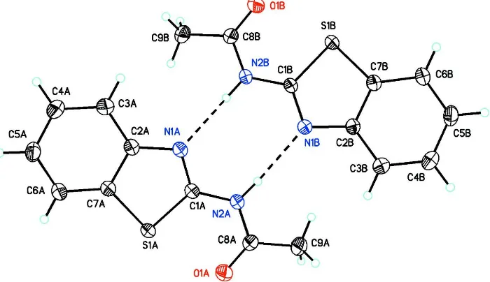
The title compound, C9H8N2OS, crystallizes with two mol-ecules (AandB) in the asymmetric unit. The dihedral angles between the mean planes of the 1,3-benzothiazol-2-yl ring system and the acetamide group are 2.7 (4) (moleculeA) and 7.2 (2) A˚ (molecule B). In the crystal, pairs of N—H N hydrogen bonds link the A and B molecules into dimers, generatingR2

2

(8) loops. The dimers stack along [100].

Related literature

For the related crystal structure of the acetamide derivatives, see: Jasinskiet al.(2013); Funet al.(2011a,b, 2012).

Experimental

Crystal data

C9H8N2OS Mr= 192.24

Monoclinic,P2₁=c a= 11.1852 (4) A˚ b= 7.4037 (4) A˚ c= 20.9189 (8) A˚

= 94.408 (3)

V= 1727.21 (13) A˚3 Z= 8

MoKradiation

= 0.33 mm 1 T= 173 K

0.450.240.15 mm

Data collection

Agilent Xcalibur (Eos, Gemini) diffractometer

Absorption correction: multi-scan (CrysAlis PROandCrysAlis RED; Agilent, 2012) Tmin= 0.770,Tmax= 1.000

20845 measured reflections 5918 independent reflections 4622 reflections withI> 2(I) Rint= 0.033

Refinement

R[F2> 2(F2)] = 0.044 wR(F2_{) = 0.109} S= 1.08 5918 reflections

237 parameters

H-atom parameters constrained

max= 0.44 e A˚ 3

min= 0.26 e A˚ 3

Table 1

Hydrogen-bond geometry (A˚ ,_).

D—H A D—H H A D A D—H A

N2A—H2A N1B 0.86 2.11 2.9700 (16) 176

N2B—H2B N1A 0.86 2.14 2.9749 (16) 165

Data collection: CrysAlis PRO(Agilent, 2012); cell refinement:

CrysAlis PRO; data reduction: CrysAlis RED (Agilent, 2012); program(s) used to solve structure: SUPERFLIP (Palatinus & Chapuis, 2007); program(s) used to refine structure:SHELXL2013

(Sheldrick, 2008); molecular graphics: OLEX2 (Dolomanovet al., 2009); software used to prepare material for publication:OLEX2.

BN thanks the UGC for financial assistance through BSR one time grant for the purchase of chemicals and DST– PURSE for financial assistance. HSY thanks University of Mysore for research facilities. JPJ acknowledges the NSF– MRI program (grant No. CHE-1039027) for funds to purchase the X-ray diffractometer.

Supplementary data and figures for this paper are available from the IUCr electronic archives (Reference: HB7144).

References

Agilent (2012). CrysAlis PRO and CrysAlis RED. Agilent Technologies, Yarnton, Oxfordshire, England.

Dolomanov, O. V., Bourhis, L. J., Gildea, R. J., Howard, J. A. K. & Puschmann, H. (2009).J. Appl. Cryst.42, 339–341.

Fun, H.-K., Loh, W.-S., Shetty, D. N., Narayana, B. & Sarojini, B. K. (2012). Acta Cryst.E68, o1348.

Fun, H.-K., Quah, C. K., Narayana, B., Nayak, P. S. & Sarojini, B. K. (2011a). Acta Cryst.E67, o2926–o2927.

Fun, H.-K., Quah, C. K., Narayana, B., Nayak, P. S. & Sarojini, B. K. (2011b). Acta Cryst.E67, o2941–o2942.

Jasinski, J. P., Guild, C. J., Yathirajan, H. S., Narayana, B. & Samshuddin, S. (2013).Acta Cryst.E69, o461.

Palatinus, L. & Chapuis, G. (2007).J. Appl. Cryst.40, 786–790. Sheldrick, G. M. (2008).Acta Cryst.A64, 112–122.

Acta Crystallographica Section E Structure Reports

Online

supporting information

Acta Cryst. (2013). E69, o1622 [doi:10.1107/S160053681302730X]

N

-(1,3-Benzothiazol-2-yl)acetamide

Prakash S Nayak, B. Narayana, Jerry P. Jasinski, H. S. Yathirajan and Manpreet Kaur

S1. Comment

In continuation of our work on the synthesis of acetamide derivatives (Jasinski et al. 2013), we report herein the crystal structure of the title compound, C9H8N2OS, (I). Some of the related crystal structures of similar acetamide derivatives

include, N-(3-chloro-4-fluorophenyl)acetamide, N-(4-bromophenyl)-2-(naphthalen-1- yl)acetamide and

N-(3,5-dichloro-phenyl)-2-(naphthalen-1-yl)acetamide (Fun et al. 2011a,b, 2012).

The title compound, (I) crystallizes with two independent molecules (A & B) in the asymmetric unit (Fig.1). The

dihedral angle between the mean planes of the 1,3-benzothiazol-2-yl ring and the acetamide group is 2.7 (4)° (A) and

7.2 (2)Å (B),(Fig. 2). In the crystal, N—H···N hydrogen bonds forming R22(8) graph set motifs which link the molecules

into dimers, which stack along [100].

S2. Experimental

2-Aminobenzothiazole (1 mmol) were dissolved in a 30 ml acetic acid and it was refluxed for 3 hrs (Fig.3). The reaction

mixture was cooled and poured into ice cold water. The precipitate obtained was obtained by filtration and recrystallized

in ethanol. Colorless blocks were grown from methanol solution by the slow evaporation method and was used as such

for X-ray studies (M.P.: 453-455 K).

S3. Refinement

All of the H atoms were placed in their calculated positions and then refined using the riding model with Atom—H

lengths of 0.93Å (CH), 0.96Å (CH3) or 0.86Å (NH). Isotropic displacement parameters for these atoms were set to 1.2

Figure 1

ORTEP drawing of (I) showing 50% probability displacement ellipsoids. Dashed lines indicate N—H···N intermolecular

hydrogen bonds between A and B forming R22(8) graph set motifs.

Figure 2

Molecular packing for (I) viewed along the b axis. Dashed lines indicate N—H···N intermolecular hydrogen bonds forming R22(8) graph set motifs which link the molecules into dimers along [100]. H atoms not involved in hydrogen

Figure 3

Synthesis scheme for (I).

N-(1,3-Benzothiazol-2-yl)acetamide

Crystal data

C9H8N2OS

Mr = 192.24

Monoclinic, P21/c

a = 11.1852 (4) Å

b = 7.4037 (4) Å

c = 20.9189 (8) Å

β = 94.408 (3)°

V = 1727.21 (13) Å3

Z = 8

F(000) = 800

Dx = 1.479 Mg m−3

Melting point: 453 K

Mo Kα radiation, λ = 0.71073 Å Cell parameters from 5326 reflections

θ = 3.3–32.7°

µ = 0.33 mm−1

T = 173 K Block, colorless 0.45 × 0.24 × 0.15 mm

Data collection

Agilent Xcalibur (Eos, Gemini) diffractometer

Radiation source: Enhance (Mo) X-ray Source Detector resolution: 16.0416 pixels mm-1

ω scans

Absorption correction: multi-scan

CrysAlis PRO and CrysAlis RED, Agilent (2012).

Tmin = 0.770, Tmax = 1.000

20845 measured reflections 5918 independent reflections 4622 reflections with I > 2σ(I)

Rint = 0.033

θmax = 32.8°, θmin = 3.3°

h = −16→16

k = −10→9

l = −30→31

Refinement

Refinement on F2

Least-squares matrix: full

R[F2 _{> 2σ(F}2_{)] = 0.044}

wR(F2_{) = 0.109}

S = 1.08 5918 reflections 237 parameters 0 restraints

Primary atom site location: structure-invariant direct methods

Hydrogen site location: inferred from neighbouring sites

H-atom parameters constrained

w = 1/[σ2_(F

o2) + (0.045P)2 + 0.4973P]

where P = (Fo2 + 2Fc2)/3

(Δ/σ)max = 0.001

Δρmax = 0.44 e Å−3

Δρmin = −0.26 e Å−3

Special details

Geometry. All esds (except the esd in the dihedral angle between two l.s. planes) are estimated using the full covariance matrix. The cell esds are taken into account individually in the estimation of esds in distances, angles and torsion angles; correlations between esds in cell parameters are only used when they are defined by crystal symmetry. An approximate (isotropic) treatment of cell esds is used for estimating esds involving l.s. planes.

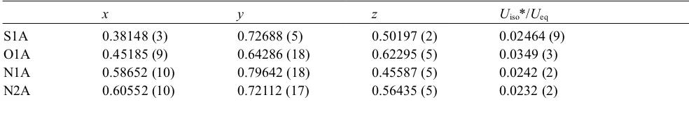
Fractional atomic coordinates and isotropic or equivalent isotropic displacement parameters (Å2₎

x y z Uiso*/Ueq

H2A 0.6815 0.7393 0.5650 0.028* C1A 0.53676 (11) 0.75086 (19) 0.50776 (6) 0.0208 (3) C2A 0.49856 (11) 0.8192 (2) 0.40579 (6) 0.0228 (3) C3A 0.51887 (13) 0.8704 (2) 0.34317 (7) 0.0301 (3) H3A 0.5961 0.8949 0.3320 0.036* C4A 0.42227 (14) 0.8841 (2) 0.29819 (7) 0.0315 (3) H4A 0.4349 0.9165 0.2563 0.038* C5A 0.30593 (13) 0.8500 (2) 0.31478 (7) 0.0303 (3) H5A 0.2423 0.8596 0.2837 0.036* C6A 0.28360 (13) 0.8024 (2) 0.37647 (7) 0.0284 (3) H6A 0.2059 0.7813 0.3876 0.034* C7A 0.38110 (12) 0.7869 (2) 0.42159 (6) 0.0225 (3) C8A 0.55898 (12) 0.6640 (2) 0.61966 (6) 0.0241 (3) C9A 0.64887 (14) 0.6310 (2) 0.67511 (7) 0.0312 (3) H9AA 0.7267 0.6141 0.6597 0.047* H9AB 0.6268 0.5247 0.6977 0.047* H9AC 0.6508 0.7329 0.7035 0.047* S1B 1.06929 (3) 0.76516 (5) 0.50481 (2) 0.02415 (9) O1B 0.99661 (9) 0.63954 (18) 0.38920 (5) 0.0338 (3) N1B 0.86730 (10) 0.77933 (17) 0.55907 (5) 0.0230 (2) N2B 0.84393 (10) 0.70106 (17) 0.45051 (5) 0.0232 (2) H2B 0.7673 0.7064 0.4517 0.028* C1B 0.91433 (11) 0.74614 (19) 0.50500 (6) 0.0200 (2) C2B 0.95787 (11) 0.8261 (2) 0.60567 (6) 0.0210 (3) C3B 0.94173 (13) 0.8677 (2) 0.66959 (7) 0.0288 (3) H3B 0.8654 0.8664 0.6844 0.035* C4B 1.04033 (14) 0.9107 (2) 0.71058 (7) 0.0316 (3) H4B 1.0302 0.9376 0.7533 0.038* C5B 1.15469 (13) 0.9140 (2) 0.68865 (7) 0.0303 (3) H5B 1.2198 0.9446 0.7169 0.036* C6B 1.17329 (12) 0.8727 (2) 0.62580 (7) 0.0273 (3) H6B 1.2499 0.8745 0.6114 0.033* C7B 1.07368 (11) 0.8283 (2) 0.58475 (6) 0.0219 (3) C8B 0.88922 (12) 0.6480 (2) 0.39429 (6) 0.0242 (3) C9B 0.79789 (13) 0.5998 (2) 0.34107 (7) 0.0300 (3) H9BA 0.7214 0.5827 0.3581 0.045* H9BB 0.8214 0.4902 0.3210 0.045* H9BC 0.7922 0.6954 0.3100 0.045*

Atomic displacement parameters (Å2₎

U11 _U22 _U33 _U12 _U13 _U23

C3A 0.0244 (7) 0.0408 (9) 0.0253 (7) 0.0003 (6) 0.0038 (5) 0.0061 (6) C4A 0.0329 (8) 0.0394 (9) 0.0222 (6) 0.0038 (6) 0.0014 (5) 0.0054 (6) C5A 0.0278 (7) 0.0382 (9) 0.0239 (6) 0.0065 (6) −0.0045 (5) −0.0010 (6) C6A 0.0201 (6) 0.0391 (9) 0.0256 (6) 0.0033 (6) −0.0010 (5) −0.0024 (6) C7A 0.0192 (6) 0.0273 (7) 0.0210 (6) 0.0017 (5) 0.0015 (4) −0.0012 (5) C8A 0.0243 (6) 0.0273 (7) 0.0206 (6) −0.0008 (5) 0.0015 (5) −0.0001 (5) C9A 0.0303 (7) 0.0387 (9) 0.0240 (7) 0.0007 (6) −0.0016 (5) 0.0046 (6) S1B 0.01533 (15) 0.0370 (2) 0.02013 (15) −0.00067 (12) 0.00165 (11) −0.00226 (13) O1B 0.0229 (5) 0.0521 (8) 0.0269 (5) −0.0017 (5) 0.0051 (4) −0.0072 (5) N1B 0.0174 (5) 0.0326 (7) 0.0190 (5) 0.0015 (4) 0.0010 (4) −0.0006 (4) N2B 0.0154 (5) 0.0346 (7) 0.0193 (5) −0.0008 (4) −0.0010 (4) −0.0007 (5) C1B 0.0154 (5) 0.0247 (7) 0.0199 (5) 0.0008 (4) 0.0002 (4) 0.0008 (5) C2B 0.0181 (6) 0.0251 (7) 0.0194 (6) 0.0021 (5) −0.0005 (4) 0.0006 (5) C3B 0.0244 (7) 0.0398 (9) 0.0223 (6) 0.0002 (6) 0.0030 (5) −0.0037 (6) C4B 0.0332 (8) 0.0413 (9) 0.0200 (6) −0.0007 (6) −0.0002 (5) −0.0040 (6) C5B 0.0277 (7) 0.0366 (9) 0.0252 (7) −0.0039 (6) −0.0065 (5) −0.0018 (6) C6B 0.0194 (6) 0.0369 (9) 0.0249 (6) −0.0025 (5) −0.0020 (5) −0.0010 (6) C7B 0.0191 (6) 0.0255 (7) 0.0209 (6) 0.0006 (5) 0.0001 (4) 0.0006 (5) C8B 0.0226 (6) 0.0297 (8) 0.0203 (6) −0.0026 (5) 0.0010 (5) −0.0004 (5) C9B 0.0310 (7) 0.0377 (9) 0.0208 (6) −0.0051 (6) −0.0014 (5) −0.0038 (6)

Geometric parameters (Å, º)

S1A—C1A 1.7407 (13) S1B—C1B 1.7392 (13) S1A—C7A 1.7390 (14) S1B—C7B 1.7333 (13) O1A—C8A 1.2156 (17) O1B—C8B 1.2157 (16) N1A—C1A 1.3018 (17) N1B—C1B 1.3068 (16) N1A—C2A 1.3913 (17) N1B—C2B 1.3945 (17)

N2A—H2A 0.8600 N2B—H2B 0.8600

N2A—C1A 1.3791 (17) N2B—C1B 1.3757 (16) N2A—C8A 1.3715 (17) N2B—C8B 1.3733 (17) C2A—C3A 1.3989 (19) C2B—C3B 1.3974 (18) C2A—C7A 1.3997 (18) C2B—C7B 1.3988 (18)

C3A—H3A 0.9300 C3B—H3B 0.9300

C3A—C4A 1.381 (2) C3B—C4B 1.381 (2)

C4A—H4A 0.9300 C4B—H4B 0.9300

C4A—C5A 1.395 (2) C4B—C5B 1.392 (2)

C5A—H5A 0.9300 C5B—H5B 0.9300

C5A—C6A 1.379 (2) C5B—C6B 1.381 (2)

C6A—H6A 0.9300 C6B—H6B 0.9300

C6A—C7A 1.3910 (19) C6B—C7B 1.3928 (18) C8A—C9A 1.4957 (19) C8B—C9B 1.4952 (19)

C9A—H9AA 0.9600 C9B—H9BA 0.9600

C9A—H9AB 0.9600 C9B—H9BB 0.9600

C9A—H9AC 0.9600 C9B—H9BC 0.9600

C1A—N2A—H2A 118.3 C1B—N2B—H2B 118.2 C8A—N2A—H2A 118.3 C8B—N2B—H2B 118.2 C8A—N2A—C1A 123.41 (12) C8B—N2B—C1B 123.62 (11) N1A—C1A—S1A 117.17 (10) N1B—C1B—S1B 117.01 (10) N1A—C1A—N2A 120.74 (12) N1B—C1B—N2B 121.32 (12) N2A—C1A—S1A 122.08 (10) N2B—C1B—S1B 121.66 (10) N1A—C2A—C3A 125.57 (12) N1B—C2B—C3B 125.69 (12) N1A—C2A—C7A 115.07 (12) N1B—C2B—C7B 115.13 (11) C3A—C2A—C7A 119.36 (12) C3B—C2B—C7B 119.18 (12) C2A—C3A—H3A 120.6 C2B—C3B—H3B 120.4 C4A—C3A—C2A 118.89 (13) C4B—C3B—C2B 119.29 (13) C4A—C3A—H3A 120.6 C4B—C3B—H3B 120.4 C3A—C4A—H4A 119.6 C3B—C4B—H4B 119.7 C3A—C4A—C5A 120.87 (13) C3B—C4B—C5B 120.63 (13) C5A—C4A—H4A 119.6 C5B—C4B—H4B 119.7 C4A—C5A—H5A 119.4 C4B—C5B—H5B 119.4 C6A—C5A—C4A 121.23 (13) C6B—C5B—C4B 121.29 (13) C6A—C5A—H5A 119.4 C6B—C5B—H5B 119.4 C5A—C6A—H6A 121.1 C5B—C6B—H6B 121.1 C5A—C6A—C7A 117.84 (13) C5B—C6B—C7B 117.86 (13) C7A—C6A—H6A 121.1 C7B—C6B—H6B 121.1 C2A—C7A—S1A 109.84 (10) C2B—C7B—S1B 109.90 (10) C6A—C7A—S1A 128.36 (11) C6B—C7B—S1B 128.35 (10) C6A—C7A—C2A 121.80 (12) C6B—C7B—C2B 121.74 (12) O1A—C8A—N2A 121.82 (13) O1B—C8B—N2B 121.45 (12) O1A—C8A—C9A 122.81 (13) O1B—C8B—C9B 123.07 (13) N2A—C8A—C9A 115.37 (12) N2B—C8B—C9B 115.48 (12) C8A—C9A—H9AA 109.5 C8B—C9B—H9BA 109.5 C8A—C9A—H9AB 109.5 C8B—C9B—H9BB 109.5 C8A—C9A—H9AC 109.5 C8B—C9B—H9BC 109.5 H9AA—C9A—H9AB 109.5 H9BA—C9B—H9BB 109.5 H9AA—C9A—H9AC 109.5 H9BA—C9B—H9BC 109.5 H9AB—C9A—H9AC 109.5 H9BB—C9B—H9BC 109.5

C3A—C4A—C5A—C6A 0.3 (3) C3B—C4B—C5B—C6B −0.7 (3) C4A—C5A—C6A—C7A −0.9 (3) C4B—C5B—C6B—C7B 0.3 (2) C5A—C6A—C7A—S1A −179.09 (13) C5B—C6B—C7B—S1B −178.14 (13) C5A—C6A—C7A—C2A 0.4 (2) C5B—C6B—C7B—C2B 0.4 (2) C7A—S1A—C1A—N1A −0.82 (12) C7B—S1B—C1B—N1B −1.16 (12) C7A—S1A—C1A—N2A 179.98 (13) C7B—S1B—C1B—N2B 177.82 (12) C7A—C2A—C3A—C4A −1.3 (2) C7B—C2B—C3B—C4B 0.2 (2) C8A—N2A—C1A—S1A 2.6 (2) C8B—N2B—C1B—S1B 7.6 (2) C8A—N2A—C1A—N1A −176.56 (14) C8B—N2B—C1B—N1B −173.46 (14)

Hydrogen-bond geometry (Å, º)

D—H···A D—H H···A D···A D—H···A