Threshold of Parametric Instability in the Ionospheric Heating
Experiments
Xiang WANG (王翔)1,2, Chen ZHOU (周晨)1,*, Moran LIU (刘默然)1, Farideh HONARY2,
Binbin NI (倪彬彬) 1, Zhengyu Zhao (赵正予) 1
1Department of Space Physics, School of Electronic Information, Wuhan University, Wuhan,
430072, People’s Republic of China
2
Department of Physics, Lancaster University, Lancaster, LA1 4YB, United Kingdom
*Corresponding author: [email protected]
Abstract
Many observations in the ionospheric heating experiment, by a powerful high frequency
electromagnetic wave with ordinary polarization launched from a ground-based facility, is
attributed to parametric instability (PI). In this paper, the general dispersion relation and the
threshold of the PI excitation in the heating experiment are derived by considering the
inhomogeneous spatial distribution of pump wave field. It is shown that the threshold of PI is
influenced by the effective electron and ion collision frequencies and the pump wave frequency.
Both collision and Landau damping should be considered in the PI calculation. The derived
threshold expression has been used to calculate the required threshold for excitation of PI for
several ionospheric conditions during heating experiments conducted employing EISCAT high
frequency transmitter in Tromsø, Norway on October 2nd 1998, November 8th 2001, October
19th 2012 and July 7th 2014. The results indicate that the calculated threshold is in good
agreement with the experimental observations.
Keywords: ionospheric plasma, ionospheric modification; parametric instability; ordinary
1 Introduction
Ionospheric modification experiments, by high powerful high-frequency electromagnetic
waves launched from the ground heating facilities, have observed many nonlinear plasma
instabilities in the past decades [1-7]. Parametric instability is directly or indirectly employed to
explain the observed phenomena during the heating experiments, such as high-frequency
enhanced ion line (HFILs), high-frequency enhanced plasma line (HFPLs) [8, 9], airglow
enhancement [10-12], stimulated electromagnetic emissions (SEEs) [13], filed-aligned
irregularities (FAIs) [14, 15], etc.
The excitation process of plasma instabilities includes a multi-wave coupling process [7,
16-20]. Two waves in the ionosphere can interact, causing perturbations to the parameters such as
current and charge density. These effects can be associated with frequency differences or
frequency sums of the two waves. Whilst a third wave, or even a fourth wave, whose frequency
equals the frequency difference or sum and whose wave vector meets the requirement of the
vector difference or sum, can be excited in the ionosphere. Ion acoustic wave/lower hybrid
wave/zero-frequency density irregularities and the Langmuir wave/upper hybrid wave are example
wave modes exist in the ionospheric plasma; an incident high power radio wave can interact with
any of these wave modes when the matching conditions of frequency and wave vectors are
satisfied.
Theoretical research of parametric instabilities in space plasma began in the 1950s by
considering nonlinear theory of wave mode transition when a Langmuir wave can decay to
who first systematically studied the process of coupling and excitation of waves in the process of
parametric instability, started from the collisionless, cold plasma fluid equations, which were
adopted only when the field strength of the incident pump wave is stronger than the threshold field.
Nishikawa [24, 25] studied the general model of exciting parameter instabilities and analyzed the
excitation of plasma waves under three conditions: (1) 1+ 2 0, (2) 12 0, (3)
1 0 2
. His results showed that the waves excited by (1) and (2) are oscillating and that
the wave of excited by (3) is non-oscillating. The equality of the threshold field can be obtained
from different methods, e.g., using the plasma hydrodynamic equations [7, 18, 24, 25], or Vlasov
equation [17, 26]. The differences between these methods are small, and they all show
proportional relation between the square of the threshold field intensity and the electron collision
frequency. Based on numerical simulations, Guzdar et al. [27] calculated the threshold field
strength of the pump wave that excites the parametric instability irregularly and found that this
threshold field strength can reach 10 V/m. Recently, Kuo [7, 18, 19] obtained a different
expression and illustrated that the square of threshold field strength is proportional to the product
of the electron and ion collision frequencies.
In this paper, MHD equations are employed to derive the parametric excitation in the
ionospheric heating experiment by a high powerful high-frequency ordinary polarized
electromagnetic wave. Equations presented here consider inhomogeneous spatial distribution of
pump wave field as well as Landau damping of Langmuir wave. In section 2, parametric
excitation in the ionosphere and its dispersion relation, as well as the dispersion relation of the
excited high frequency sidebands and the low frequency decay mode are calculated when the
instability threshold indicates that both collision and Landau damping terms are needed to explain
the experimental observations in section 3, followed by the conclusion and summary in section 4.
2 Theory
2.1 Excitation of parametric instability
Ionospheric heating experiments have shown that Langmuir waves/upper hybrid wave and
ion acoustic waves/lower hybrid wave can be excited in the ionospheric modification [7, 9, 28, 29].
The pump wave
(
)
p 0, 0
E k could be either an electromagnetic (EM) wave or an electrostatic (ES)
wave. It was hypothesized that the oscillations of the main modes in the plasma are
(
k, )
and,
(
kd = k,
d =
)
, In general, this excitation process includes a four-wave coupling process;which it will reduce to a three-wave coupling process under certain conditions. This process
requires a wave vector and frequency matching condition:
0 d d
=
++
=
−−
(1)0 d d
k
=
k
++
k
=
k
−−
k
(2)where the subscripts 0, +, - andd represent the pump wave, the down-shifted high frequency mode,
the up-shifted high frequency mode and the low frequency decay mode, respectively.
The dispersion relation for the parametric instability is derived from the following equations:
Continuity Equation
(
)
α α α
0
n
t
n v
+
=
(3)Momentum Equations:
(
)
(
)
e e e e e e e
3
e e e e e em n
+
t
v
r v
= −
en E
+
v
B
+
en
−
T
n
−
m n
v
(4a)(
)
(
)
i i i i i i i i i i i i i i i
m n
+
t
v
r v
=
e n E
+
v
B
−
e n
−
T
n
+
m n v
(4b)2
α α 0
e n
= −
(5)where the subscript
α
refers toe
andi
, the electron and ion, respectively.n
α,m
α,e
α,T
αand
v
α are the density, mass, charge, temperature, and speed of particleα
, respectively.E
is the electric field strength;B
is the magnetic field;
is the potential of the plasma wave;
0 is the free space permittivity; and electron and ion effective collision frequencies are given bye ei en eL
=
+
+
and
i=
ie+
in+
iL, respectively, where
ei,
en,
eL,
ie
in andiL
are electron-ion collision frequency, electron-neutral collision frequency, electron Landaudamping rate, ion-electron collision frequency, ion-neutral collision frequency and ion Landau
damping rate, respectively.
The incident pump wave field is assumed to be:
(
)
0
k
exp
0 02
E
=
E
i k r
−
t
(6)The perturbation of the incident pump field is assumed to be small, meaning that the magnitude of
the intensity of the excited plasma waves is far less than that of the pump wave. The density of
charged particles satisfies the quasi-neutrality condition, i.e.
n
0e=
n
0i=
constant
. Every physicalquantity is treated as the sum of frequency components, for example,
(k ,ω0 0) ( k, ω) ( k, ω)
v
=
v
+
v
+
v
, where the subscript is the exponent, likewise,( k, ω) k
exp
(
)
kexp
(
)
v
=
v
i k r
−
t
+
v
−
−
i k r
−
t
. The physical quantities describedby frequency components are incorporated into the original equations and the terms of the same
exponent are combined. The arbitrariness of
r
andt
demands that the coefficient of eachexponent term is equal to zero. Thus, a series of equations of frequency components can be
obtained to determine the dispersion relation of the wave coupling. Finally, the excitation
equation.
To begin with, let us consider the geomagnetic field
B
0=
B z
0ˆ
and the wave numberk
0of the heater wave is much smaller than the wave numbers of the electrostatic, i.e.
k
0
0
. First of all, we simplify the equations concerning the(
+ +
k
0,
0)
wave mode. The momentum equation can be reduced to:0 0 0
e k e k k
e
ˆ
2
e
V
V
z
E
t
m
+
+
= −
(7)The cross product of the k0 component of Eq. (7) with
z
ˆ
is taken as:(
0)
0 0e k e k k
e
ˆ
ˆ
2
e
V
z
V
E
z
t
⊥m
+
−
= −
(8)Take the perpendicular component of Eq. (7) into Eq. (8),
(
0)
0 02 2
e e k e k e k
e e
ˆ
ˆ
2
2
e
e
V
z
E
E
z
t
m
⊥t
m
+
+
= −
−
+
(9)Substitute Eq. (9) into Eq. (7)
0
0 0 0
2 2
e e e k
2
2
e k e k z e e k e
ˆ
2
V
t
t
e
E
E
E
z
m
t
t
+
+
+
=
−
+
+
−
+
(10)Equation (10) can be written as a scalar equation in the
k
−
domain to obtain the expression of 0 kV
:(
)
(
)
(
) (
)
0 0 0
0
2 2
0 e k e k z 0 e e k
k 2
2
e 0 e 0 e e
ˆ
2
e
i
E
E
i
i
E
z
V
i
m
i
i
+
−
−
+
= −
+
+
−
(11)where
=
eeB m
0 e is the electron cyclotron frequency.In the high frequency sideband wave field, only electron can respond to the wave field due to
of the high frequency sideband plasma wave excited by parametric instability can be obtained
(
)
(
)
(
)
(
) (
)
(
(
)
)
( )
(
)
(
)
(
)
(
) (
)
(
)
(
)
2 2 e e 22 2 2 4
e 0 e p e pz
2 2
2 2 2 2 2 2 2 2
2
0 e 0 e e 0 e e p
2 2 2 2
e
0 e p
2 2
2 2 2
2 2 2 2 2 2
e e Te pe k
2 2
2 2
0 e 0 e e
2 2 e 2 e e 3 sin cos ˆ ˆ
i i k v n
i k k
k k E E E z e z k i
m i E
+ − + − − − − + + + + + + − + + + + + − + = + +( )
(
)
(
)(
)
(
)
(
)
0 0
k
2 2
e e z k e e k Δk
e
* p
2 2 2 *
0 e e p ˆ p
ˆ 2
n
k k
e
i i k k E i k E z n
E z E
m E
⊥ + + − − + + − − + (12)where
pe2=
(
n e
0 2
0m
e)
,(
)
e
2
T b e e
v
=
k T m
are the electron plasma frequency, and theelectron thermal speed, respectively and
k
b is the Boltzmann constant. The term in the left-hand side of Eq. (12) defines the dispersion relation of the excited high frequency plasma wave; whilethe terms in the right-hand side are the coupling terms driving the plasma waves. The first term in
the right-hand side is caused by the spatial non-uniformity of the wave field and the second term
indicates the coupling between the pump wave and the lower frequency decay mode, which
influences the excitation of the high frequency Langmuir wave/ upper hybrid wave sideband. The
ratio of the two terms in the right-hand side of Eq. (12) is close to 1; which indicates that the
nonlinear force generated by the non-uniform spatial wave field is important in the excitation of
parametric instability.
Finally, the dispersion relation of the low frequency decay mode can be analyzed in the
following manner. Both the electron and the ion contribute to the low frequency plasma wave field.
For simplification, electrons and ions assume to maintain quasi-neutrality in the low frequency
(
)
(
)
(
)
(
)
(
)
(
)
(
) (
)
(
(
)
)
( )
(
)
2
2 2 4
0 e p e pz
2 2
2 2 2 2 2 2 2
0 e 0 e e 0 e
2 2 2 2 2
e e i s
Δk 2
2 2 2 2 i 2
i e s e i
e
2 2
2 2 2
e e
e i
cos
sin 1 cot 1 cot
cos
i i k c
n m
i i k c
m
i k k
m m E E − − + + − + + = − + + + − − + − + + + + + + − + + + −
(
)
(
)
(
) (
)
(
(
)
)
(
(
)( )
)(
)
(
)
(
0)(
)
(
)
(
0)
2
e p
2
2 2 *
0 e p p
2 2 2 2 2 *
2 2 2 2 2
0 e e p p
0
2
Δk
e e
2 2
e e 0 k k e e 0 k
e i
e 0 e e
ˆ si ˆ ˆ n E z E E
E z E
k
n
k z k
i i
k k
i n k V k V i i n k V
m m ⊥ + + − − + + − + + + + + + − +
(
)
(
) (
)
(
)
(
)
(
)
(
)
0 0 k 2 2e e e k k
2 2 2 2
k
e e e e k
e
ˆ
cos sin
2
k V z
i i k V n
en
i i i ik E
m + + − + + + − + + + + (13)
where
c
s2=
k T
b(
e+
3
T
i)
m
i is the ion acoustic wave phase speed, =
ieB m
0 i is the ion cyclotron frequency,
is the angle between the wave vectork
and the magnetic fieldB
0;(
)
(
)
(
) (
)
2 2
e e z e e
k
k 2 2 2
0
e e e e
ˆ
e
i
i
z en
V
k
m
i
i
−
+ −
−
= +
−
−
+
, which is the linear part of theelectron velocity response to the high frequency plasma wave field. The terms in the left-hand side
of Eq. (13) defines the dispersion relation of the excited low frequency decay mode in the
parametric instability. The right-hand side of Eq. (13) illustrates the coupling terms driven the
parametric instability. The pump wave and the high frequency sidebands couple with each other to
exert a low frequency nonlinear force on electrons and to make the coupling waves grow
significantly in the expense of the pump wave.
2.2 Instability Threshold
In this section, excitation of parametric instability by an ordinary polarized electromagnetic
pump wave in the ionospheric modification experiments is considered. In this condition, the
O-mode pump wave
E
p(
k
0,
0)
decays to a Langmuir/upper hybrid sidebandn
k(
k
,
)
the reflection height of the pump wave. In terms of the wave frequency and wave vector matching
condition, i.e. Eq. (1) and (2), the following expression of the frequency and wave vector are
obtained:
= =
0−
,k
+= − = −
k
−k
, wherez
ˆ
ˆ
k
=
k z
+
k x
⊥ (14)The pump wave field can be expressed as
(
)
0 0
p
ˆ
k2
ˆ
ˆ
k2
E
=
z E
+
x iy E
+
(15)In the following, Eq. (12) and (13) with the aid of Eq. (14) and (15) are analyzed to explain
excitation of parametric instabilities for different scenarios.
2.2.1 Parametric instability near the O-mode wave reflection height
When the ordinary polarized EM wave propagates to the region near the reflection altitude,
the electric field of the pump wave is
(
)
(
)
0
p
ˆ
k2 cos
0E
=
z E
−
i
t
. Then the expressions for0
k
V
,V
k,(
) (
)
0
* k
k
kV
V
k
, and(
) (
)
0 0
* k
k
kV
V
k
reduce to(
0)
0
k k
e 0 e
2
eE
V
i
m
i
=
+
(16a)(
)
2
pe k
k 2
e 0
k
n
V
k
i
n
=
+
(16b)
(
0) (
)
(
(
)
)
0 0
*
k k
2 2
k 2 2 2 e 0 e
4
e
k E
k
k
m
V
V
=
+
(16c)
(
)(
)
(
0)
0
2 pe k
* k
k k 2 2
0 e 0 e
2
e
k E
n
k V
k V
i
n
m
=
+
(16d)
Considering a case when the pump wave decay to a Langmuir wave and an ion acoustic wave,
the process reduces to a three-wave interaction, i.e. a pump wave, a Langmuir wave and an ion
(
)
(
)
(
(
)
)
2 2 2 2 2 2
e Te pe e k
2 2
e e
1 2 2 k
2 2
0 e 2
e e
3
sin
1
1
cos
i
k v
n
i
i
n
i
−
−
+
+
+
+
−
+
−
+
+
= +
(17)(
)
(
)
(
)(
)
2 2 e
i s k
i e
1
2 2 2
pe 0 e k
i
e e 0
m
i
k c
n
m
m
n
m
i
i
i
+
−
+
+
+
=
−
−
+ +
(18)where
(
)
(
)
0
2 2
k e 0 e
1
e k E
2
m
=
+
,(
)
(
)
0
2
2 2 2 2
k
4
e 0 ee
k E
m
=
+
.From Eq. (17) and Eq. (18), the dispersion relation for PDI can be obtained:
(
)
(
)
(
)
(
)
(
p2 2 2)
(
)(
)
2 2 2 2 2 2 2 2
e
e
e Te pe e i s
i 2 2 e e e e 2
2 2 0 e 0 e
i e e
3
sin
1
1
cos
m
i
k v
i
k c
m
i
m
i
m
i
i
−
−
+
+
+
+ −
+
+
+
−
+
= −
+ +
−
+
−
−
−
(19)By setting
=
Re
( )
+
i
, =
Re
( )
+
i
,k
=
kz
ˆ
, when the growth rate0
=
, the threshold of PDI in the steady can be written as3 2 2 2
2 i e 0 e i e 0
th 2 2 2 2 2 2 2
0 pe e 0
4
1
cos
cos
1
m m
E
e k
−
=
+
−
(20)where
=
kc
s.For the case when pump wave decays into two Langmuir waves with purely growing mode,
e.g. when the oscillation two-stream instability, is excited near the reflection height of the pump
wave, the two oppositely propagating Langmuir waves and a zero-frequency purely growing mode
are excited by the pump wave. The frequency of the Langmuir wave and purely growing mode are
set as
=
0+
i
and =
i
, respectively. The threshold expression becomes(
)
(
)
(
(
)
)
2 2 4 2 2 2 2 2
s 0 1 0 e e 0
2 e i
th 2 2 2 2 2 2 2
1 0 pe e 0
1
cos
2
cos
1
c
m m
E
e
+
−
=
+
−
(21)when the growth rate
is 0; where
12=
02−
3
k v
2 2Te−
pe2−
e2sin
2
.When the right-hand polarized electromagnetic wave plays its role as a pump wave, it can
reach an altitude where the upper hybrid frequency equals the pump wave frequency, called ‘the
upper hybrid resonant height. In this region, the electric field of the ordinary polarized pump wave
is
(
)
(
)
(
)
0
p
ˆ
ˆ
k2 cos
0E
=
x iy
+
E
−
i
t
.Then the expressions for
0
k
V
,V
k,(
) (
)
0 0
* k
k
kV
V
k
, and(
)(
)
0
*
k k
k V
k V
reduce to(
0)
0
k k
e 0 e e
2
eE
V i
m i
=
− +
(22a)
(
)
2 pe k k 2 0 e e k n V n k i = − +
(22b)
(
) (
)
(
(
0)
)
0 0 2 2 k 2 2 2 e * 0 e k e k 4
e k E
k k m V V = − +
(22c)
(
)(
)
(
(
)
0)
0
2 pe k
* k
k k 2
2 2
0
e 0 e e
2
e k E n
k V k V i
n m k = − +
(22d)
For a case when the pump wave decays to an upper hybrid wave and a lower hybrid wave
near the upper hybrid resonant region of the pump wave. The threshold for
=
0
can be writtenas
(
)
22 4
e 0 e e i
2 0 e 2 e
th 4 2
0 b e pe i 0
4
1
cot
1
3
m n
m
E
k T k
m
+
=
+
−
(23)by setting the frequency of
=
Re
( )
+
i
,
= +
i
, andk
=
kx
ˆ
into Eq. (12) and (13).When the pump wave excites the oscillating two-stream instability near the O-mode upper
hybrid resonant region, the two upper hybrid waves
(
k
=
kx
ˆ,
)
and a field-aligned purely growing mode(
= −
k
kx
ˆ,
=
i
)
are involved. In this case, the threshold expression is:(
)
(
)
(
)
2 2 2 2 2 2 2
pe Te e 0 0 b e i
2
th 2 2
0 pe T e 0 e e i
4
3
1
3
3
1
k
k
T
T
v
E
n
v
k
+
+ −
+
+
=
3. Comparison with experimental observations
In this section, threshold calculations have been performed for different experiments
conducted at Tromsø, Norway. The relevant ionospheric parameters are provided by EISCAT
website (http://www.eiscat.se/madrigal). The neutral densities and collision frequencies are
obtained from NRLMSISE-00 [30] and the geomagnetic field strength is obtained from the
International Geomagnetic Reference Field (IGRF11) [31].
Four different experiments are considered as listed in Table 1. The experiments on 19th
October, 2012 and 7th July, 2014 operated at daytime, and the experiments on 8th November, 2001 and on 2nd October, 1998 ran at nighttime. All these experiments operated with the different heater wave frequency due to the different ionospheric conditions. The effective radiated powers (ERP)
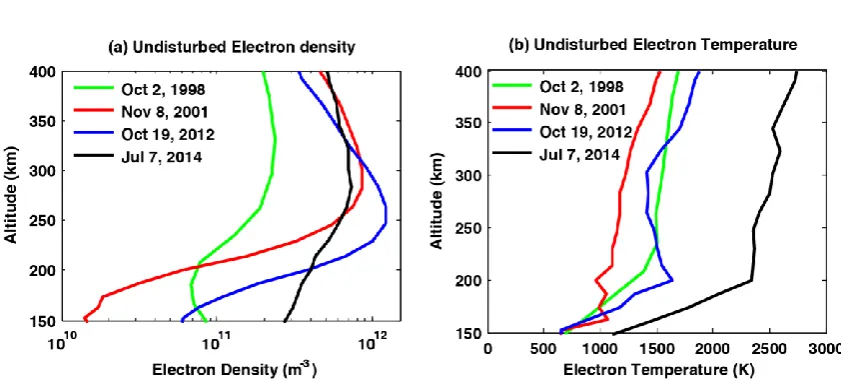
listed in the Table 1 take into account the D-region absorption [32]. Figure 1 illustrates the
unperturbed electron temperature and electron density profile for these four experiments, which
are obtained from the measurement of the undisturbed ionosphere before the heater was turned on.
The experiments were chosen to represent both day and night conditions as well as different
background electron temperature and electron density. For example, for the two nighttime
experiments, the electron density for the experiment on 2nd October, 1998 is much smaller
compared to the experiment conducted on 8th November, 2001; whereas the electron temperature
is 50% higher in 2nd October, 1998 experiment compared to the experiment on 8th November,
2001. The two daytime experiments of 19th October, 2012 and 7th July, 2014 show similar difference in the electron density and temperature, i.e. higher electron density with lower electron
temperature. In the interaction region, the background electron density and electron temperature in
experiments provide different conditions to calculate the PI threshold as indicated in Table 1 and
Figure 1. The unperturbed ionospheric parameters for these four experiments, with aid of
NRLMSISE-00 and IGRF model, were used to calculate the threshold and the equivalent ERP of
parametric instability as presented in the last eight rows in Table 1. The wave number in the
calculation is taken as 12.44π, which is twice the wave number of the 930 MHz UHF radar at
[image:13.595.88.512.277.748.2]Tromsø.
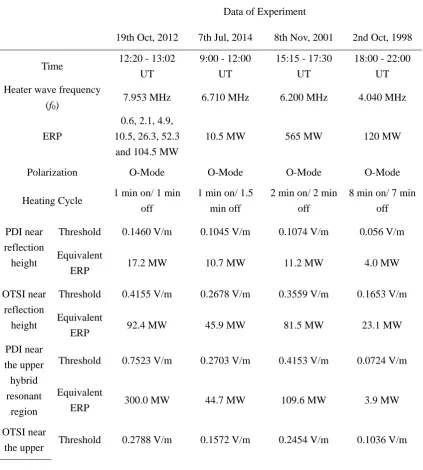
Table 1 The experiments setting and PI threshold
Data of Experiment
19th Oct, 2012 7th Jul, 2014 8th Nov, 2001 2nd Oct, 1998
Time 12:20 - 13:02
UT
9:00 - 12:00 UT
15:15 - 17:30 UT
18:00 - 22:00 UT Heater wave frequency
(f0)
7.953 MHz 6.710 MHz 6.200 MHz 4.040 MHz
ERP
0.6, 2.1, 4.9, 10.5, 26.3, 52.3
and 104.5 MW
10.5 MW 565 MW 120 MW
Polarization O-Mode O-Mode O-Mode O-Mode
Heating Cycle 1 min on/ 1 min
off
1 min on/ 1.5 min off
2 min on/ 2 min off
8 min on/ 7 min off
PDI near reflection height
Threshold 0.1460 V/m 0.1045 V/m 0.1074 V/m 0.056 V/m
Equivalent
ERP 17.2 MW 10.7 MW 11.2 MW 4.0 MW
OTSI near reflection
height
Threshold 0.4155 V/m 0.2678 V/m 0.3559 V/m 0.1653 V/m
Equivalent
ERP 92.4 MW 45.9 MW 81.5 MW 23.1 MW
PDI near the upper hybrid resonant
region
Threshold 0.7523 V/m 0.2703 V/m 0.4153 V/m 0.0724 V/m
Equivalent
ERP 300.0 MW 44.7 MW 109.6 MW 3.9 MW
OTSI near
hybrid resonant
region
Equivalent
ERP 41.3 MW 15.1 MW 38.3 MW 8.1 MW
Figure 1. (a) undisturbed electron density profile, and (b) undisturbed electron temperature profiles during the Ionospheric modification experiments; the different colors indicate the different
experiments.
For the experiment on 19th Oct, 2012, the downshifted HFILs which indicate the excitation of
PDI appear in the ion line spectral when the ERP reached 26.3 MW and the zero-offset HFILs
shows when ERP achieved 52.3 MW, which is the signature of the OTSI [33]. Therefore,
indicating that the PDI can be excited when the ERP range is from 10.5 MW to 26.3 MW; and the
ERP of the excitation of OTSI is within a range of 26.3 MW to 52.3 MW. The lack of observation
of HFILs in the ion spectral for 7th July 2014 experiment indicates that the parametric instability
was not excited, and there was no obvious heating effect in this experiment. The lack of the PI
excitation and heating can be explained by the presence of high electron density in the E-region
and consequent high absorption of the pump wave power before reaching the interaction height.
The two nighttime experiments displayed intense airglow enhancement and HFILs in the ion line
spectra manifesting the excitation of the parametric instability [34, 35].
When the parametric instability is excited near the pump wave reflection height, the threshold
[image:14.595.89.510.123.314.2]2 times higher threshold than PDI. Both these threshold values for PDI and OTSI are well within
the ERP that can be achieved by the Tromsø heating facility. The threshold depends on the
effective collision frequencies of charged particles, electron density and electron and ion
temperature. Thus, the difference in the PDI threshold for the experiment on 7th July, 2014 compared to the experiment on 19th October, 2012 is due to the difference in electron temperature. As it can be seen from Figure 1, the background electron temperature was high during the
experiment of 7th July, 2014, resulting in a high threshold value. The effective collision
frequencies of the electron and ion decrease with the growth of the temperature which
significantly influences the threshold value. The difference of the thresholds in the nighttime
experiments compared to the daytime experiments can also be explained due to the electron
temperature difference.
When the parametric instability occurs near the pump wave upper hybrid resonant region, the
threshold is related to the wavelength of the plasma wave, which is associated with the transvers
width of the irregularities. The backscatter UHF radar cannot detect the upper hybrid waves
excited by the parametric instability; thus, in this paper, it’s assumed that the wave number of
upper hybrid wave is twice the wave number of the 930 MHz UHF radar. The threshold of
parametric instability is considerably influenced by the scale of the irregularities, due to the
relation between wavelength and wave number k=2 .
3.1 Comparison with other PDI threshold calculation reported in the literature
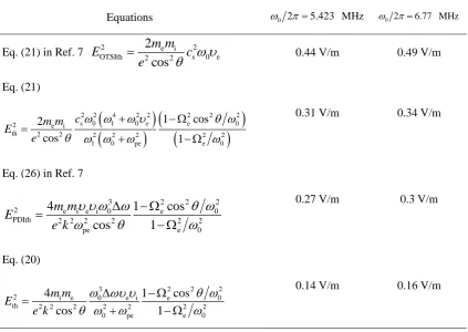
The results presented in section 2 are compared with the results presented in Kuo’s paper [7].
The relevant parameters of the HF heating experiments conducted at Tromsø, Norway have been
i 1000 K
T = ,
in=0.8 s−1 ,v
Te=
1.5 10
5m s
, 2Ti 7.17 10 m s
v = ,
3
s 1.52 10 m s
c = , 4 1
iL 1.19 10 s
= − , 1e 600 s
= − ,
=
12
. The threshold valuesestimated by Eq. (20) and (21) in this paper are compared to Eq. (21) and Eq. (25) in Ref. 7 and
[image:16.595.88.512.229.529.2]listed in the Table 2.
Table 2. Comparison of the threshold evaluations
Equations 0 2=5.423 MHz 0 2 =6.77 MHz
Eq. (21) in Ref. 7 OTSIth2 2
2
e 2i s2 0 ecos
m m
E
c
e
=
0.44 V/m 0.49 V/mEq. (21)
(
)
(
)
(
(
)
)
2 2 4 2 2 2 2 2
s 0 1 0 e e 0
2 e i
th 2 2 2 2 2 2 2
1 0 pe e 0
1 cos
2
cos 1
c m m E
e
+ −
=
+ −
0.31 V/m 0.34 V/m
Eq. (26) in Ref. 7
3 2 2 2
2 e i e i 0 e 0
PDIth 2 2 2 2 2 2
pe e 0
4
1
cos
cos
1
m m
E
e k
−
=
−
0.27 V/m 0.3 V/m
Eq. (20)
3 2 2 2
2 i e 0 e i e 0
th 2 2 2 2 2 2 2
0 pe e 0
4 1 cos
cos 1
m m E
e k
−
=
+ −
0.14 V/m 0.16 V/m
As illustrated in Table 2, the PDI threshold value near the pump wave reflection height
calculated by the equations in Kuo’s paper [7] are higher by nearly a factor of 2 compared to our
results; also, for the OTSI, Kuo’s result is approximately 1.4 times more than the threshold values
obtained using the derived equations in this paper. For the experiment performed on 19th October
2012, the Langmuir PDI had been excited when ERP reached 26.3 MW; but 10.5 MW ERP cannot
excite parametric decay instability, i.e. the equivalent ERP of the threshold value range of PDI is
from 10.5 MW to 26.3 MW. We have calculated the PDI threshold value and equivalent ERP using
paper [7]. The threshold of PDI using Eq. (26) in Kuo’s paper [7] is 0.204 V/m and the equivalent
ERP is 33.7 MW, which are higher than the experimental observation.
4. Summary
In the present study the excitation of plasma waves due to high-frequency electromagnetic
wave heating in the ionosphere are discussed. Equations that describe the threshold field of pump
waves for the excitation of parametric instability have been derived. The results are also compared
with the experiments operated with EISCAT heating facility. Our study indicates that the threshold
field of the excited parametric instability is proportional to the product of the electron collisions
frequency and the ion collisions frequency, including the effects of the Landau damping, which
plays important roles in the threshold estimation. Our results also demonstrate that the OTSI
requires higher threshold than PDI, which is consistent with the experimental observations. In the
dispersion relation of the excited high frequency sideband and low frequency decay mode, the
coupling terms in right hand side of Eq. (12) and Eq. (13) drive the excited plasma wave modes.
The first term of the right-hand side arises from the spatial non-uniformity of the high frequency
wave, which cannot be neglected in the excitation process. Therefore, using the threshold
expression derived in this paper and comparing with results of previous research as indicated in
Table 2 illustrates that the inclusion of the inhomogeneity of the pump wave field are important
and need to be considered when evaluating the threshold of PDI in order to explain experimental
observations.
Acknowledgments
EISCAT is an international scientific association supported by research organizations in
United Kingdom (NERC). This work was supported by the National Natural Science Foundation
of China (NSFC grants 41204111, 41574146, 41774162 and 41704155) and China Postdoctoral
Science Foundation (2017M622504). The data used in this paper are available through the
EISCAT Madrigal database (http://www.eiscat.se/madrigal/).
References
[1] Utlaut W F and Cohen R 1971 Science174 245
[2] Grach S M and Trakhtengerts V Y 1975 Radiophys. Quantum El. 18 951
[3] Minkoff J et al 1974 Radio Sci9 941
[4] Robinson T R 1989 Phys. Rep. 179 79
[5] Stubbe P 1996 J. Atmos. Terr. Phys.58 349
[6] Leyser T B and Wong A Y 2009 Rev. Geophys.47 514
[7] Kuo S P 2015 Phys. Plasmas22 012901
[8] Frey A 1986 Geophys. Res. Lett.13 438
[9] Rietveld M T et al 2000 J. Geophys. Res.105 7429
[10] Bernhardt P A et al 1989 J. Geophys. Res.94 9071
[11] Kosch M J, et al 2002 Geophys. Res. Lett.29 27
[12] Kosch M J et al 2007 J. Geophys. Res.112 A06325
[13] Stubbe P et al 1984 J. Geophys. Res.89 7523
[14] Thome G D and Blood D W 1974 Radio Sci.9 915
[15] Frolov V L et al 2014 Radiophys. Quantum El.57 393
[17] Fejer J A 1979 Rev. Geophys.17 135
[18] Kuo S P 1996 Phys. Plasmas3 3957
[19] Kuo S P 2014 Pr Electromagn Res.60 141
[20] Kuo S P et al 1983 J. Geophys. Res.88 417
[21] Gekker I R 1982 The interaction of strong electromagnetic fields with plasmas Clarendon
Press Oxford
[22] Silin V P 1965 Sov. Phys. JETP21 1510
[23] Silin V P 1968 Proc. Eighth Int. Conf. Phenom Ionized Gases 205
[24] Nishikawa K 1968 J. Phys. Soc. Jpn. 24 916
[25] Nishikawa K 1968 J. Phys. Soc. Jpn.24 1152
[26] Fejer J A and Leer E 1972 J. Geophys. Res.77 700
[27] Guzdar P N et al 1996 J. Geophys. Res.101 2453
[28] Tzoar N 1969 Phys. Rev.178 356
[29] Utlaut W F and Violette E J 1972 J. Geophys. Res.77 6804
[30] Picone J M et al 2002 J. Geophys. Res.107 1468
[31] Finlay C C et al 2010 Geophys. J. Int.183 1216
[32] Senior A et al 2010 J. Geophys. Res.115 A09318
[33] Bryers C J et al 2013 J. Geophys. Res.118 7472
[34] Blagoveshchenskaya N F et al 2005 Ann. Geophys.23 87