https://doi.org/10.1007/s11222-019-09903-y
Sequential Monte Carlo with transformations
Richard G. Everitt1 ·Richard Culliford2·Felipe Medina-Aguayo2·Daniel J. Wilson3
Received: 17 December 2018 / Accepted: 3 September 2019 © The Author(s) 2019
Abstract
This paper examines methodology for performing Bayesian inference sequentially on a sequence of posteriors on spaces of different dimensions. For this, we use sequential Monte Carlo samplers, introducing the innovation of using deterministic transformations to move particles effectively between target distributions with different dimensions. This approach, combined with adaptive methods, yields an extremely flexible and general algorithm for Bayesian model comparison that is suitable for use in applications where the acceptance rate in reversible jump Markov chain Monte Carlo is low. We use this approach on model comparison for mixture models, and for inferring coalescent trees sequentially, as data arrives.
Keywords Bayesian model comparison·Coalescent·Trans-dimensional Monte Carlo
1 Introduction
1.1 Sequential inference
Much of the methodology for Bayesian computation is designed with the aim of approximating a posteriorπ. The most prominent approach is to use Markov chain Monte Carlo (MCMC), in which a Markov chain that hasπas its limiting distribution is simulated. It is well known that this process may be computationally expensive; that it is not straight-forward to tune the method automatically; and that it can be challenging to determine how long to run the chain for. There-fore, designing and running an MCMC algorithm to sample from a particular targetπmay require much human input and computer time. This creates particular problems if a user is
The authors gratefully acknowledge funding from BBSRC, the Wellcome Trust, the Royal Society and the Modernising Medical Microbiology group.
Electronic supplementary material The online version of this article (https://doi.org/10.1007/s11222-019-09903-y) contains
supplementary material, which is available to authorized users.
B
Richard G. Everitt1 Department of Statistics, University of Warwick, Coventry
CV4 7AL, UK
2 Department of Mathematics and Statistics, University of
Reading, Reading, UK
3 Nuffield Department of Medicine, University of Oxford,
Oxford, UK
in fact interested in a number of target distributions(πt)Tt=1 defined possibly on different spaces: using MCMC on each target requires additional computer time to run the separate algorithms and each may require human input to design the algorithm, determine the burn in, etc. This paper has as its subject the task of using a Monte Carlo method to simulate from each of the targetsπtthat avoids these disadvantages.
Particle filtering (Gordon et al.1993) and its generalisa-tion, the SMC sampler (Del Moral et al.2006) is designed to tackle problems of this nature. Roughly speaking, the idea of these approaches is to begin by using importance sampling (IS) to find a set of weightedparticlesthat give an empirical approximation toπ0then to, fort =0, ...,T−1, update the set of particles approximatingπtsuch that they, after chang-ing their positions uschang-ing a kernel Kt+1and updating their weights, approximateπt+1. This approach is particularly use-ful where neighbouring target distributions in the sequence are similar to each other, and in this case has the following advantages over runningT separate MCMC algorithms.
– When the targets(πt)Tt=1are only known up to a constant of proportionality, SMC samplers also provide unbiased estimates of the corresponding normalising constants. In a Bayesian context, the normalising constant of πt is the marginal likelihood or evidence, a key quantity in Bayesian model comparison. For much of the paper, and in abuse of notation, we use the same letters for denot-ing distributions and corresponddenot-ing densities. In addition, we use tildes to denote unnormalised densities; e.g., let
θ∼πt(·)then its density is given byπt(θ)= ˜πt(θ) /Zt, whereZtdenotes the normalising constant.
1.2 Outline of paper
In this paper, we consider the case where eachπtis defined on a space of different dimension, often of increasing dimension witht. We provide a general framework for implementing an SMC algorithm in the aforementioned setting. A particle fil-ter is designed to be used in a special case of this situation: the case whereπtis the path distribution in a state space model, πt(θ1:t|y1:t). A particle filter exploits the Markov property in order to update a particle approximation ofπt(θ1:t|y1:t) to an approximation ofπt+1(θ1:t+1|y1:t+1). In this paper, we consider targets in which there is not such a straight-forward relationship betweenπt andπt+1. In addition, the approach we present is useful in Bayesian model comparison that results from constructing an SMC sampler where eachπt corresponds to a different model and there areT models that can be ordered, usually in order of their complexity. Deter-ministic transformations are used to move points between one distribution and the next, potentially yielding efficient samplers by reducing the distance between successive distri-butions. We also show how the same framework can be used for sequential inference under the coalescent model (King-man1982).
The use of deterministic transformations to improve SMC has been considered previously in a number of papers (e.g., Chorin and Tu2009; Vaikuntanathan and Jarzynski 2011; Reich2013; Heng et al.2015; South et al.2019). Several of these papers are focussed on how to construct useful trans-formations in a generic way including, for example: methods that map high density regions of the proposal to high den-sity regions of the target (Chorin and Tu2009) and methods that approximate the solution of ordinary differential equa-tions that mimic the SMC dynamics (Heng et al.2015). This paper is different in that it focuses on the particular case of a sequence of distribution on spaces of different dimensions, and uses transformations and proposals that are designed for the applications we study.
Section2 describes the methodology introduced in the paper, considering both practical and theoretical aspects, and provides comparison to existing methods. We provide an example of the use of the methodology for Bayesian model
comparison in Sect. 3, on the Gaussian mixture model. In Sect.4, we use our methodology for online inference under the coalescent, using the flexibility of our proposed approach to describe a method for moving between coalescent trees. In Sect.5, we present a final discussion and outline possible extensions.
2 SMC samplers with transformations
2.1 SMC samplers with increasing dimension
The use of SMC samplers on a sequence of targets of increas-ing dimension has been described previously (e.g., Naesseth et al.2014; Everitt et al.2017; Dinh et al.2018). These papers introduce an additional proposal distribution for the variables that are introduced at each step. In this section, we straight-forwardly see that this is a particular case of the SMC sampler in Del Moral et al. (2007).
2.1.1 SMC samplers with MCMC moves
To introduce notation, we first consider the standard case in which the dimension is fixed across all iterations of the SMC. For simplicity, we consider only SMC samplers with MCMC moves, and we consider an SMC sampler that has T itera-tions. Letπt be our target distribution of interest at iteration
t, this being the distribution of the random vectorθton space
E. Throughout the paper, the values taken by particles in the SMC sampler have a(p)superscript to distinguish them from random vectors; so for exampleθt(p)is the value taken by the
pth particle. We defineπ0to be a distribution from which we can simulate directly, simulate each particleθ0(p) ∼π0and set its normalised weightw(0p)=1/P. Then for 0≤t <T
at the(t+1)th iteration of the SMC sampler, the following steps are performed.
1. ReweightCalculate the updated (unnormalised) weight
˜ w(p)
t+1of the pth particle
˜ w(p)
t+1=w( p) t
˜ πt+1
θ(p)
t
˜ πt
θ(p)
t
. (1)
2. ResampleNormalise the weights to obtain normalised weights wt(+p)1 and calculate the effective sample size
(ESS) (Kong et al.1994). If the ESS falls below some threshold, e.g.,αPwhere 0< α <1, then resample. 3. MoveFor each particle use an MCMC move with target
We remark that the move step above does not necessarily imply using a single MCMC iteration; if the chosen MCMC mixes slowly then performing many iterations and using adaptive strategies will result beneficial. The previous algo-rithm yields an empirical approximation ofπtand an estimate of its normalising constantZt
ˆ πP
t = P
p=1 w(p)
t δθ(p) t ,
Zt = t
s=0 P
p=1 w(p)
s ˜ πs+1
θ(p)
s
˜ πs
θ(p)
s
(2)
whereδθ is a Dirac mass atθ.
2.1.2 Increasing dimension
We now describe a case where the parameterθincreases in dimension with the number of SMC iterations. Our approach is to set up an SMC sampler on an extended space that has the same dimension of the maximum dimension ofθthat we will consider [similarly to Carlin and Chib (1995)]. At SMC iterationt, we use:θtto denote the random vector of interest;
ut to denote a random vector that contains the additional dimensions added to the parameter space at iterationt+1, andvtto denote the remainder of the dimensions that will be required at future iterations. Our SMC sampler is constructed on a sequence of distributionsϕt of the random vectorϑt = (θt,ut, vt)in spaceE=(Θt,Ut,Vt), with
ϕt(ϑt)=πt(θt) ψt(ut|θt) φt(vt|θt,ut) , (3)
whereπt is the distribution of interest at iterationt, andψt andφt are (normalised) distributions on the additional vari-ables so thatπt andϕt have the same normalising constant. The weight update in this SMC sampler is
˜ w(p)
t+1=w( p) t
˜ πt+1
θ(p)
t ,u( p) t ˜ πt θ(p)
t
ψt
u(tp)|θ( p) t
. (4)
Here, as in particle filtering, by construction, theφtterms in the numerator and denominator have cancelled so that none of the dimensions added after iterationt+1 are involved; a characteristic shared by the MCMC move with targetϕt+1, that need only updateθt,ut.
2.2 Motivating example: Gaussian mixture models
2.2.1 RJMCMC for Gaussian mixture models
The following sections make use of transformations and other ideas in order to improve the efficiency of the sampler. To motivate this, we consider the case of Bayesian model com-parison, in which theπtare different models ordered by their complexity. In Sect.3, we present an application to Gaussian
mixture models, and we use this as our motivating example here. Consider mixture models withtcomponents, to be esti-mated from datay, consisting ofNobserved data points. For simplicity, we describe a “without completion” model, where we do not introduce a labelzthat assigns data points to com-ponents. Let thesth component have a meanμs, precision τsand weightνs, with the weights summing to one over the components. Letpμandpτbe the respective priors on these parameters, which are the same for every component, and let
pν be the joint prior over all of the weights. The likelihood undertcomponents is
ft
y|θt =(μs, τs, νs)ts=1
= N
i=1 t
s=1 νsN
yi|μs, τs−1
.
(5)
An established approach for estimating mixture models is that of RJMCMC. Here,tis chosen to be a random variable and assigned a prior pt, which here we choose to be uniform over the values 1 toT. Let
πt(θt)=π (θt|t,y)
∝ pν(ν1:t) t
s=1
pμ(μs)pτ(τs)
ft
y|θt=(μs, τs, νs)ts=1
(6)
be the joint posterior distribution over the parametersθt con-ditional on t. RJMCMC simulates from the joint space of
(t, θt) in which a mixture of moves is used, some fixed-dimensional (t fixed) and some trans-dimensional (to mix overt). The simplest type of trans-dimensional move in this case is that of a birth move for moving fromttot+1 compo-nents or a death move for moving fromt+1 tot(Richardson and Green1997). We consider a birth move, a uniform prior probability overt and equal probability of proposing birth or death. For the purposes of exposition, we assume that the weights of the components are chosen to be fixed in each model. (This assumption will be relaxed later in Sect. 3.) Letut =(μt+1, τt+1), be the mean and precision of the new component and letψt(ut|θt)=pμ(μt+1)pτ(τt+1). A birth move simulatesut ∼ψtand has acceptance probability
α=min
1, πt+1(θt+1)
πt(θt) ψt(ut|θt)
, (7)
whereθt+1=(θt,ut).
2.2.2 Comparing RJMCMC and SMC samplers
vt =
μ(t+2):T, τ(t+2):T
and
φt(vt|θt,ut)= T
s=t+2
pμ(μs)pτ(τs) ,
we may use the SMC sampler described in Sect.2.1.2. Note that the ratio in the acceptance probability in Eq. (7) is the same as the incremental SMC weight in Eq. (4). The reason for this is that both algorithms make use of an IS estimator of the Bayes factorZt+1/Zt: using a proposed pointθt ∼πt,
ut ∼ψt andθt+1=(θt,ut), this estimator is given by
Zt+1
Zt =
πt+1(θt+1) πt(θt) ψt(ut|θt).
(8)
We may see RJMCMC as using an IS estimator of the ratio of the posterior model probabilities within its accep-tance ratio; this view on RJMCMC (Karagiannis and Andrieu 2013) links it to pseudo-marginal approaches (Andrieu and Roberts2009) in which IS estimators of target distributions are employed. As in pseudo-marginal MCMC, the efficiency of the chain depends on the variance of the estimator that is used. We observe that the IS estimator in Eq. (8) is likely to have high variance: this is one way of explaining the poor acceptance rate of dimension changing moves in RJMCMC. In particular, we note that this estimator suffers a curse of dimensionality in the dimension ofθt+1, meaning that RJM-CMC is in practice seldom effective when the parameter space is of high dimension. This view suggests a number of potential improvements to RJMCMC with a birth move, each of which has been previously investigated.
– IS performs better if the proposal distribution is close to the target, whilst ensuring that the proposal has heavier tails than the target. The original RJMCMC algorithm allows the possibility to construct such proposals by allowing for the use of transformations to move from the parameters of one model to the parameters of another. Richardson and Green (1997) provide a famous example of this in the Gaussian mixture case in the form of split-merge moves. Focusing on the split move, the idea is to propose splitting an existing component, using a moment matching technique to ensure that the new components have appropriate means, variances and weights.
– Annealed importance sampling (AIS) (Neal2001) yields a lower variance than IS. The idea is to use intermediate distributions to form a path between the IS proposal and target, using MCMC moves to move points along this path. This approach was shown to be beneficial in some cases by Karagiannis and Andrieu (2013).
– The estimator in Eq. (8) uses only a single importance point. It would be improved by using multiple points.
However, using such an estimator directly within RJM-CMC leads to a “noisy” algorithm that does not have the correct target distribution for the same reasons as those given for the noisy exchange algorithm in Alquier et al. (2016). We note that recent work (Andrieu et al. 2018) suggests a correction to provide an exact approach based on the same principle.
The approach we take in this paper is to investigate varia-tions on these ideas within the SMC sampler context, rather than RJMCMC. We begin by examining the use of trans-formations in Sect.2.3, then describe the use of intermediate distributions and other refinements in Sect.2.4. The final idea is automatically used in the SMC context, due to the use of
Pparticles.
2.3 Using transformations in SMC samplers
We now show (in a generalisation of Sect.2.1.2) how to use transformations within SMC, whilst simultaneously chang-ing the dimension of the target at each iteration; an approach we will refer to astransformation SMC(TSMC). We again use the approach of performing SMC on a sequence of tar-getsϕt, with each of the these targets being on a space of fixed dimension, constructed such that they have the desired targetπt as a marginal. In this section, the dimension of the space on whichπt is defined again varies witht, but is not necessarily increasing witht. Letθtbe the random vector of interest at SMC iterationt: we wish to approximate the distri-butionsπtofθtin the spaceΘt. Let(ϕ˜t)Tt=1be a sequence of unnormalised targets, whose normalised versions are(ϕt)Tt=1 and being the distribution of the random vectorϑt =(θt,ut) in the spaceEt =(Θt,Ut)where
˜
ϕt(θt,ut)= ˜πt(θt) ψt(ut|θt) ,
implyingϕt andπt have the same normalising constantZt. The dimension ofΘt can change witht, but the dimension of Et must be constant int. We introduce a transformation
Gt→t+1:Θt×Ut →Θt+1×Ut+1and define
ϑt→t+1=(θt→t+1(ϑt) ,ut→t+1(ϑt)):=Gt→t+1(ϑt) .
In many cases, we will chooseGt→t+1to be bijective. In this case, we denote its inverse byGt+1→t =G−t→1t+1, with
ϑt+1→t =(θt+1→t(ϑt+1) ,ut+1→t(ϑt+1)) :=Gt+1→t(ϑt+1) .
Let the distribution of the transformed random variable
These distributions may be derived using standard results about the distributions of transforms of random variables: e.g., where theEt are continuous spaces and whereGt→t+1 is a diffeomorphism, having Jacobian determinantJt→t+1, with inverseGt+1→t having Jacobian determinant Jt+1→t. In this case we have
˜
ϕt→t+1(ϑt→t+1)= ˜πt(θt+1→t(ϑt→t+1))
×ψt(ut+1→t(ϑt→t+1)|θt+1→t(ϑt→t+1))|Jt+1→t|, ˜
ϕt+1→t(ϑt+1→t)= ˜πt+1(θt→t+1(ϑt+1→t))
×ψt+1(ut→t+1(ϑt+1→t)|θt→t+1(ϑt+1→t))|Jt→t+1|.
We may then use an SMC sampler on the sequence of targets
ϕt, with the following steps at its(t+1)th iteration.
1. Transform For the pth particle, apply ϑt(→p)t+1 =
Gt→t+1
ϑ(p) t
.
2. Reweight and resampleCalculate the updated (unnor-malised) weightw˜(t+p)1
˜ w(p)
t+1=w( p) t
˜ ϕt+1
ϑ(p)
t→t+1
˜ ϕt→t+1
ϑ(p)
t→t+1
. (9)
WhereGt→t+1is a diffeomorphism we have
˜ w(p)
t+1=w (p) t
˜ πt+1
θ(p)
t→t+1
ψt+1
u(t→p)t+1|θt(→p)t+1
˜ πt
θ(p)
t
ψt
u(tp)|θ( p) t
|Jt+1→t| .
(10)
It is possible, depending on the transformation used, that this weight update involves none of the dimensions above max{dim(θt) ,dim(θt+1)} as happened in (4). Then resample if the ESS falls below some threshold, as described previously.
3. Move For each p, letϑt(+p)1 be the result of an MCMC move with targetϕt+1, starting fromϑt(→p)t+1. We need not simulateuvariables that are not used at the next iteration.
To illustrate the additional flexibility this framework allows, over and above the sampler described in Sect.2.1.2, we con-sider the Gaussian mixture example in Sect.2.2. The sampler from2.1.2provides an alternative to RJMCMC in which a set of particles is used to sample from each model in turn, using the particles from modelt, together with new dimen-sions simulated using a birth move, to explore modelt+1. The sampler in this section allows us to use a similar idea using more sophisticated proposals, such as split moves. The efficiency of the sampler depends on the choice ofψt and
Gt→t+1. As previously, a good choice for these quantities
should result in a small distance betweenϕt→t+1andϕt+1, whilst ensuring thatϕt→t+1has heavier tails thanϕt+1. As in the design of RJMCMC algorithms, usually these choices will be made using application-specific insight.
2.4 Design of SMC samplers
2.4.1 Using intermediate distributions
The Monte Carlo variance of an SMC sampler depends on the distance between successive target distributions; thus, a well-designed sampler will use a sequence of distributions in which the distance between successive distributions is small. We ensure this by introducing intermediate distributions in between successive targets (Neal2001): in between targets
ϕtandϕt+1we useK−1 intermediate distributions, thekth beingϕt,k, so thatϕt,0=ϕt andϕt,K =ϕt+1and therefore ϕt,K =ϕt+1,0. We usegeometric annealing, i.e.,
˜ ϕt→t+1,k
ϑt→t+1,k
=ϕ˜t+1
ϑt→t+1,k γk
˜ ϕt→t+1
ϑt→t+1,k 1−γk
, (11)
where 0 = γ0 < ... < γK = 1. This idea results in only small alterations to the TSMC presented above. We now use a sequence of targets ϕt,k, incrementing the t index when
k = K, then settingk = 0 and finally using a transform moveϑt(→p)t+1,0=Gt→t+1
ϑ(p)
t,K
for eachp∈ {1, . . . ,P}. The weight update becomes
˜ w(p)
t,k+1=w (p) t,k
˜
ϕt→t+1,k+1
ϑ(p) t→t+1,k
˜ ϕt→t+1,k
ϑ(p)
t→t+1,k
, (12)
and the MCMC moves now have targetϕt→t+1,k+1, starting fromϑt(→p)t+1,kand storing the result inϑt(→p)t+1,k+1. The use of intermediate distributions makes this version of TSMC more robust than the previous one; the MCMC moves used at the intermediate distributions provide a means for the algo-rithm to recover if the initial transformation is not enough to ensure thatϕt→t+1is similar toϕt+1.
2.4.2 Adaptive SMC
CESSt,k+1=
PPp=1w(t,pk)ω(p)
2
P p=1w(
p) t,k
ω(p)2 , (13)
to monitor the discrepancy between neighbouring distribu-tions, whereω(p)is the incremental weight given by the ratio multiplyingw(t,pk)in (12). Before the reweighting step is per-formed, the next intermediate distribution is chosen to be the distribution under which the CESS is found to beβP, for some 0< β < 1. In the case of the geometric anneal-ing scheme, this corresponds to a particular choice forγk for computing (11). As commented previously, we may also adapt the MCMC kernels used for the move step, based on the current particle set. For the two examples presented later, we have considered adaptive and non-adaptive strategies in the MCMC kernels. We refer the interested reader to the supplementary material for the specific details. Algorithm1 presents a generic version of TSMC using adaptive resam-pling and number of intermediate distributions.
2.4.3 Auxiliary variables in proposals
For the Gaussian mixture example, for two or more com-ponents, when using a split move we must choose the component that is to be split. We may think of the choice of splitting different components as offering multiple “routes” through a space of distributions, with the same start and end points. Another alternative route would be given by using a birth move rather than a split move. In this section, we gener-alise TSMC to allow multiple routes. We restrict our attention to the case where the choice of multiple routes is possible at the beginning of a transition fromϕt toϕt+1, whenk =0 (more general schemes are possible). A route corresponds to a particular choice for the transformationGt→t+1; thus, we consider a set ofMtpossible transformations indexed by the discrete random variablelt, using the notationG(tl→t)t+1(also using this superscript on distributions that depend on this choice ofG). We now augment the target distribution with variablesl0, ...,lT−1and, for eacht alter the distributionψt such that it becomes a joint distribution onut andlt. Our sampler will draw thel variables at the point at which they are introduced, so that different particles use different routes, but will not perform any MCMC moves on the variable after it is introduced. This leads to the sampler being degenerate in most of thelvariables, but this doesn’t affect the desired target distribution.
A revised form of TSMC is then, whenk = 0, to first simulate routeslt(p) ∼ ρt for each particle, then to use a
different transformϑt(→p)t+1,0 = G
l(tp)
t→t+1
ϑ(p) t,K
dependent on the route variable. The weight update is then given by
˜ w(p)
t+1=w( p) t
˜ πt+1
θ(p)
t→t+1
ψt+1
u(t→p)t+1,lt(p)|θ( p) t→t+1
˜ πt
θ(p)
t
ψt
u(tp),l( p) t |θ(
p) t J
lt(p)
t+1→t
,
(14)
where for simplicity we have omitted the dependence ofu(tp),
ut(→p)t+1andθt(→p)t+1onlt(p). This weight update is very similar to one found in Del Moral et al. (2006), for the case where a discrete auxiliary variable is used to index a choice of MCMC kernels used in the move step. Analogous to Del Moral et al. (2006), the variance of (14) is always greater than or equal to that of (10); we present an example in Sect. 3 where this additional variance can result in large errors in marginal likelihood estimates). Alternatively one can employ the Rao– Blackwellisation procedure found in population Monte Carlo (Douc et al.2007) and marginalise the proposal over the aux-iliary variablelt. This results in a weight update of
˜ w(p)
t+1=w (p) t
πt+1
θ(p) t→t+1
ψt+1
u(t→p)t+1|θt(→p)t+1
Mt
m=1πt
θ(p) t
ψt
u(tp),m|θ( p) t J(
m) t+1→t
. (15)
As mentioned in Del Moral et al. (2006), using (15) comes with extra computational cost, which could be prohibitively large ifMt is large.
Algorithm 1: TSMC algorithm with adaptive resam-pling and intermediate distributions
Input: Particle approximation{ϑt(p), w(
p)
t }Pp=1≈ϕt; ESS
thresholdα∈(0,1); CESS thresholdβ∈(0,1).
Output: Particle approximation{ϑt(+p)1, wt(+p)1}Pp=1≈ϕt+1;
EstimatorZt+1/Zt.
1 Initialisek=0,γk =0,Z:=Zt+1/Zt=1.
2 foreachp∈ {1, . . . ,P}do
3 Transform particleϑt(→p)t+1,k=Gt→t+1(ϑt(p)).
4 Setw(t,pk)=w(tp).
5 whileγk<1do
6 Findγk+1∈(0,1]such thatC E S St,k+1=βP.
7 foreachp∈ {1, . . . ,P}do
8 Compute the weightw˜(t,pk)+1using (12).
9 UpdateZ=ZPp=1w˜(t,pk)+1.
10 Renormalise the above weights to obtain{wt(,pk)+1}Pp=1. 11 ifE S St,k+1< αPthen
12 Resample particles an setw(t,pk)+1=1/Pfor all p∈ {1, . . . ,P}.
13 foreachp∈ {1, . . . ,P}do
14 Setϑt(→p)t+1,k+1∼Kt,k+1(ϑt(→p)t+1,k,·), whereKt,k+1is a
ϕt→t+1,k+1-invariant MCMC kernel.
2.5 Discussion
One of the most obvious applications of TSMC is Bayesian model comparison. SMC samplers are a generalisation of several other techniques, such as IS, AIS and the “stepping stone” algorithm from Xie et al. (2011) (which is essentially equivalent to AIS where more than one MCMC move is used per target distribution); thus, we expect a well-designed SMC to outperform these techniques in most cases. Zhou et al. (2015) reviews existing techniques that use SMC for model comparison and concludes that “the SMC2 algorithm (mov-ing from prior to posterior) with adaptive strategies is the most promising among the SMC strategies.” In Sect.3, we provide a detailed comparison of TSMC with SMC2 and find that TSMC can have significant advantages.
Section2.2.2 compared TSMC with RJMCMC, noting that RJMCMC explores the model space by using a high variance estimator of a Bayes factor at each MCMC itera-tion, whereas TSMC is designed to construct a single lower variance estimator of each Bayes factor. The high vari-ance estimators within RJMCMC are the cause of its most well-known drawback: that the acceptance rate of trans-dimensional moves can be very small. The design of TSMC, in which each model is visited in turn, completely avoids this issue. One might envisage that despite avoiding poor mixing, TSMC might instead yield high variance Bayes factor esti-mators for challenging problems. However, TSMC has the advantage that that adaptive methods may be used in order to reduce the possibility that the estimators have high variance by, for example, automatically using more intermediate dis-tributions. The possibility to adaptively choose intermediate distributions also provides an advantage over the approach of Karagiannis and Andrieu (2013), where a sequence of inter-mediate distributions for estimating each Bayes factor must be specified in advance.
Since, by construction, TSMC is a particular instance of SMC as described in Del Moral et al. (2006), all of the the-oretical properties of a standard SMC algorithm apply. Of particular interest are the properties of the method as the dimension of the parameter spaces grows. TSMC is con-structed on a sequence of extended spacesEt, each of which has dimensiondT, thus in the worst case, the results for an SMC sampler on a space of dimension dT apply. In this respect, the authors in Beskos et al. (2014) have analysed the stability of SMC samplers as the dimension of the state space increases when the number of particles P is fixed. Their work provides justification, to some extent, for the use of intermediate distributionsϕt,k
K
k=1. Under fairly strong assumptions, it has been shown that when the number of intermediate distributions K = O(dT), and asdT → ∞, the effective sample size ESStP+1 is stable in the sense that it converges to a non-trivial random variable taking val-ues in(1,P). The total computational cost for bridgingϕ
and ϕt+1, assuming a product form of dT components, is
OPdT2. However, in practice, due to the cancellation of “fill in” variables, and using sensible transformations between consecutive distributions, one could expect a much lower effective dimension of the problem; an example of this sit-uation is presented in the next section. Some theoretical properties of the method are explored further in the Sup-plementary Information.
3 Bayesian model comparison for mixtures
of Gaussians
In this section, we examine the use of TSMC on the mix-ture of Gaussians application in Sect. 2.2: i.e., we wish to perform Bayesian inference of the number of components
t, and their parametersθt, from data y. For simplicity, we study the “without completion” model, where component labels for each measurement are not included in the model. In the next sections, we outline the design of the algorithms used, then in Sect.3.2we describe the results of using these approaches on previously studied data, highlighting features of the approach. Further results are given in the Supplemen-tary Information.
3.1 Description of algorithms
Lett be the unknown number of mixture components, and
(μ1:t, τ1:t, ν1:t)(means, precisions and weights respectively) be the parameters of thetcomponents. Our likelihood is the same as in Eq. (5); we use priorsτ ∼Gamma2,2S2/100,
ν1:t ∼ Dir(1, ...,1)for the precisions and weights, respec-tively, and for the means we choose an unconstrained prior ofμ∼Nm,S2, wheremis the mean andS is the range of the observed data. We impose an ordering constraint on the means, as described in Jasra et al. (2005), which simpli-fies the problem by eliminating many posterior modes with the added benefit of improving the interpretability of our results. For simplicity, we have also not included the com-monly used “random beta” hierarchical prior structure onτ (Richardson and Green1997), which from a statistical per-spective is suboptimal but which simplifies our presentation of the behaviour of TSMC.
transformation in TSMC. Full details of the transformations, weight updates and MCMC moves are given in the Supple-mentary Information. In summary, we use the birth and split moves referred to in Sect. 2.2, together with a move that orders the components. For both moves, we present results using the weight updates in Eqs. (14) (referred to hence-forth as the conditional approach) and (15) (referred to as the marginal approach).
3.2 Results
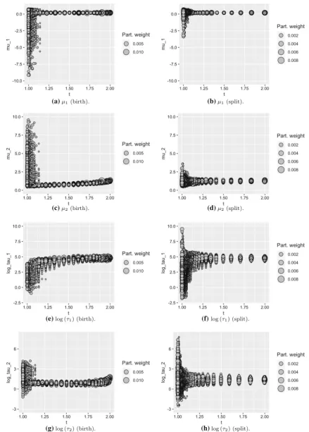
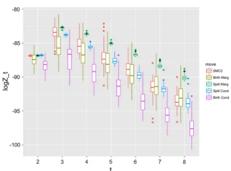
We ran SMC2 and the TSMC approaches on the enzyme data from Richardson and Green (1997). We ran the algorithms 50 times, up to a maximum ofT =8 components, withP=500 particles. We used an adaptive sequence of intermediate dis-tributions, choosing the next intermediate distribution to be the one that yields a CESS (Eq.13) ofβP, whereβ =0.99. We resampled using stratified resampling when the ESS falls belowαP, whereα=0.5. Figure1compares the birth and split TSMC algorithms when moving from one to two com-ponents. We observe that the split transformation has the effect of moving the parameters to initial values that are more appropriate for exploring the posterior on two com-ponents. For this dataset, the birth move is a poor choice for the existing parameters in the model: Fig.1e shows that no particles drawn from the proposal (i.e., the posterior for the single component model) overlap with the posterior for the first component in the two component model. Despite the poor proposal, the intermediate distributions (of which there are many more than used for the split move) enable a good representation of the posterior distribution, although below we see that the poor proposal results in very poor estimates of the marginal likelihood.
Figure2a shows log marginal likelihood estimates from the different approaches (note that a poor quality SMC usually results in an underestimate of the log marginal likelihood), and the cumulative number of intermediate dis-tributions used in estimating all of the marginal likelihoods up to modelt for eacht ∈ {1, . . . ,T}. We observe that the performance of SMC2 degrades as the dimension increases due to the increasing distance of the prior from the pos-terior: we see that the adaptive scheme using the CESS results in the number of intermediate distributions across all dimensions being approximately constant which, as sug-gested by Beskos et al. (2014) is insufficient to control the variance as the dimension grows. As discussed above, both birth TSMC methods yield inaccurate Bayes’ factor estimates, with split TSMC exhibiting substantially bet-ter performance. However, we see that neither conditional approach yields very accurate results when using the weight update given in Eq. (14); instead the marginalised weight update is required to provide good estimates. The marginal version of split TSMC significantly outperforms the other
approaches, although we note that this is achieved at a higher computational cost due to the sum in the denomina-tor of the weight updates, this can be observed in Fig.2c which shows the cumulative number of Gaussian evalua-tions for computing the weights in each case. For all TSMC approaches, we see that the number of intermediate distri-butions (Fig.2b) decreases as we increase dimension. This result can be attributed to the relatively small change that results from only adding a single component to the model at a time in TSMC. If the method has a good representation of the target at modeltand there is minimal change in the pos-terior on the existingt components when moving to model
t+1, then the SMC is effectively only exploring the posterior on the additional component and thus has higher ESS.
In the Supplementary Information, we provide similar results for two other datasets, stressing that sensible trans-formations and efficient MCMC moves are essential for obtaining good estimates of the normalising constants. Inter-estingly, and in contrast to the enzyme data presented above, for one of these other datasets neither the split nor the birth moves outperformed SMC2; this is due to the specific distri-bution of the observations in such dataset.
4 Sequential Bayesian inference under the
coalescent
4.1 Introduction
(a)μ1(birth). (b)μ1(split).
(c)μ2(birth). (d)μ2(split).
(e)log (τ1) (birth). (f)log (τ1) (split).
τ2) (birth).
(g)log ( (h)log (τ2) (split).
[image:9.595.76.516.52.666.2](a)Box plots of the log marginal likelihood estimates from each algorithm. Black dots represent the “truth” computed using a long SMC2 run.
(b)The cumulative number of intermediate distributions up to model t.
(c)The cumulative number of Gaussian evaluations needed for computing the incremental weights up to model t.
Fig. 2 The relative performance of the different SMC schemes on the mixture example
routinely in population genetics, such as the infinite variance harmonic mean estimator (Drummond and Rambaut2007) and the stepping stone algorithm (Drummond and Rambaut 2007; Xie et al.2011).
4.1.1 Previous work
The idea of updating a tree by adding leaves dates back to at least Felsenstein (1981), in which he describes, for maxi-mum likelihood estimation, that an effective search strategy in tree space is to add species one by one. More recent work also makes use of the idea of adding sequences one at a time: ARGWeaver (Rasmussen et al.2014) uses this approach to initialise MCMC on (in this case, a space of graphs),t +1 sequences using the output of MCMC ont sequences, and TreeMix (Pickrell and Pritchard2012) uses a similar idea in a greedy algorithm. In work conducted simultaneously to our own, Dinh et al. (2018) also propose a sequential Monte Carlo approach to inferring phylogenies in which the sequence of distributions is given by introducing sequences one by one. However, their approach: uses different proposal distribu-tions for new sequences; does not infer the mutation rate simultaneously with the tree; does not exploit intermediate distributions to reduce the variance; and does not use adaptive MCMC moves. Further investigation of their approach can be found in Fourment et al. (2018), where different guided proposal distributions are explored but that still presents the aforementioned limitations.
4.1.2 Data and model
We consider the analysis ofTaligned genome sequencesy= y1:T, each of lengthN. Sites that differ across sequences are known as single nucleotide polymorphisms (SNPs). The data (which is freely available fromhttp://pubmlst.org/saureus/) used in our examples consists of seven “multi-locus sequence type” (MLST) genes of 25Staphylococcus aureussequences, which have been chosen to provide a sample representing the worldwide diversity of this species (Everitt et al.2014). We make the assumption that the population has had a constant size over time, that it evolves clonally and that SNPs are the result of mutation. Our task is to infer the clonal ancestry of the individuals in the study, i.e., the tree describing how the individuals in the sample evolved from their common ancestors, and [additional to Dinh et al. (2018)] the rate of mutation in the population. We describe a TSMC algorithm for addressing this problem in Sect.4.2, before presenting results in Sect.4.3. In the remainder of this section, we intro-duce a little notation.
[image:10.595.55.288.49.221.2]πt(Tt, θ|y1:t)∝ f (y1:t|Tt, θ)p(Tt)p(θ)
fort =1:T. We here we use the coalescent prior (Kingman 1982) p(Tt)for the ancestral tree, the Jukes-Cantor substi-tution model (Jukes and Cantor1969) for f (y1:t|Tt, θ)and choose p(θ)to be a gamma distribution with shape 1 and rate 5 (that has its mass on biologically plausible values of
θ). Letl(ta)denote the length of time for whicha branches exist in the tree, for 2≤ a ≤ t. The heights of the coales-cent events are given byh(a) =ιt=alt(ι), withh(
a)
t being the (t−a+1)th coalesence time when indexing from the leaves of the tree. We letTt be a random vector
Bt,h(t2), ...,h( t) t
whereBt is itself a vector of discrete variables representing the branching order. When we refer to a lineage of a leaf node, this refers to the sequence of branches from this leaf node to the root of the tree.
4.2 TSMC for the coalescent
In this section, we describe an approach to adding a new leaf to an existing tree, using a transformation as in Sect.2.3. The basic idea is to first propose a lineage to add the new branch to (from distributionχt(g)), followed by a heighth(tnew)
conditional on this lineage (from distributionχt(h)) at which the branch connected to the new leaf will join the tree. The resultant weight update is
˜
wt+1=wtπ
t+1(Tt+1, θ|y1:t+1) πt(Tt, θ|y1:t)
s∈Λ
χ(g)
t (gt =s|θt,Tt,y1:t+1)
×χ(h) t
h(tnew)|gt =s, θt,Tt,y1:t+1 (16)
whereΛis the set that contains the leaves of the lineages that if proposed, could have resulted in the new branch (under the inverse image of the transformation). Note the relationship with Eq. (15): we achieve a lower variance through summing over the possible lineages rather than using an SMC over the joint space that includes the lineage variable.
To choose the lineage, we make use of an approximation to the probability that the new sequence is Ms mutations from each of the existing leaves, via approximating the pair-wise likelihood of the new sequence and each existing leaf. Following Stephens and Donnelly (2000) (see also Li and Stephens (2003)), we set the probability of choosing the lin-eage with leafsusing
χ(g)
t (s|θt,y1:t+1)∝
Nθt
t+Nθt Ms
. (17)
Forχt(h), we propose to approximate the pairwise like-lihood ft+1,s
ys,yt+1|θ,ht(new),gt =s
, where ys is the
sequence at the leaf of the chosen lineage. Since only two sequences are involved in this likelihood, it is likely to have heavier tails than the posterior. We use a Laplace approxima-tion on a transformed space, following Reis and Yang (2011): further details are given in the Supplementary Information, Sect.3.2.
4.3 Results
We used P = 250 particles, with an adaptive sequence of intermediate distributions, choosing the next intermediate distribution to be the one the yields a CESS (Eq.13) ofβP, where β = 0.95. Resampling is performed whenever the ESS falls belowαP, whereα = 0.5. At each iteration we used the current population of particles to tune the proposal variances, as detailed in the Supplementary Information, sec-tion 3.3.
We used six different configurations of our approach, for two different orderings of the 25 sequences. The two orderings were chosen as follows: the “nearest”/“furthest” ordering was chosen by starting with the two sequences with the smallest/largest pairwise SNP difference, then add sequences in the order of minimum/maximum SNP differ-ence to an existing sequdiffer-ence. The six configurations of the methods were: the default configuration; using no tree topol-ogy changing MCMC moves; takingχt(h) to be an Exp(1) distribution (less concentrated than the Laplace-based pro-posal); raising Eq. (17) to the power 0 to give a uniform lineage proposal; raising Eq. (17) χt(g) to the power 2; and raising Eq. (17)χt(g) to the power 4. These latter two approaches use a lineage proposal where the probability is more concentrated on a smaller number of lineages.
Figure 3 shows majority-rule consensus trees from an MCMC run and the final TSMC iterations. Figure3b is gener-ated by the default configuration (for the “furthest” ordering, although results from the “nearest” ordering are nearly iden-tical) and is close to the ground truth in Fig.3a (as determined by a long MCMC run). Figure3c, d used no topology chang-ing MCMC moves, thus illustratchang-ing the contribution of the SMC proposal in determining the topology. Table1shows estimates of the log marginal likelihood from each configu-ration of the algorithm for both orderings (longer runs of our method suggest the true value is≈ −6333), along with the total number of intermediate distributions used. Recall that a poorer-quality SMC usually results in an underestimate of the log marginal likelihood, and the number of intermediate distributions offers an indication as to the distance between the target and the proposal where the proposal has heavier tails than the target. We draw the following conclusions:
MLST97
MLST59
MLST123 ML
ST34
MLST36
MLST151
MLST6
MLST15
MLST239
MLST5
MLST133
MLST105
MLST20 MLST30
MLST1 MLST101
MLST39
MLST22
MLST25 MLST88
MLST250 MLST93 MLST45
MLST398
MLST8
(a)MCMC using 50 million iterations.
MLST239 ML
ST93
MLST20
MLST3
4
MLST8 8
MLST250
MLST398
MLST5 MLST39
MLST45
MLST25
MLST8
MLST59
MLST97 MLST6
MLST22
MLST10 5
MLST101
MLST151
ML ST
1
MLST123 MLST36
MLST30
MLST133
M LST15
(b) Default configuration using “nearest” ordering.
MLST151 MLST398
ML ST101
MLST30 MLST93
MLST25
MLST239
MLST39
MLST250
MLST88
MLST36
MLST22 MLST133
MLST20
MLST8
MLST123
MLST15 MLST105
MLST59
ML ST1
MLST97
MLST6
MLST5
MLST34
MLST45
(c) No topology moves using “furthest” ordering.
MLST59
MLS T25 MLST398
MLST88
MLST123
MLST6
MLST133
MLST239
MLST1
MLST5 MLST22
8 T S L M
MLST30
MLS T101
MLST93
MLST105
ML ST45
MLST39
MLS T15
MLST20 ML
S T97
ML ST151
MLST36 M
LST
34
MLST250
(d) No topology moves using “nearest” ordering.
[image:12.595.58.542.51.568.2]Fig. 3 Majority-rule consensus trees found by MCMC and the default configuration of TSMC (top), and different configurations of TSMC (bottom) with differences to the result obtained by the default configuration highlighted
Table 1 Log marginal likelihood estimates and total number of distributions for TSMC applied to the coalescent (5 s.f.), for the “Furthest” (first line) and “Nearest” (second line) orderings
Default No top. moves χt(h)=Exp(1) χt(h)0 χt(h)2 χt(h)4
−6333.9/267 −6338.8/257 −6335.1/408 −6336.9/330 −6333.1/247 −6334.3/238
[image:12.595.48.547.635.690.2]“nearest” ordering. “Furthest” provides an ordering in which new sequences are often added above the root of the current tree, since the existing sequences are all more closely related than the new sequence, whereas “nearest” frequently results in adding a leaf close to the existing leaves of the tree. In the latter strategy, the pro-posal relating to the new sequence is often good, but adding a new sequence can have a large effect on the posterior of existing variables. We see this by comparing Fig.3c, d, observing that the “furthest” ordering results in a topology that is close to the truth. The topology from the “nearest” ordering is not as close to the truth, thus is more reliant on topology changing MCMC moves to give an accurate sample from the posterior.
– As expected, using no MCMC topology moves results in very poor estimates, highlighting the important role of MCMC in generating diversity not introduced in the SMC proposals. This poor quality is not accounted for by the adaptive scheme based on the CESS introducing more intermediate distributions, since the CESS is only based on the weights of the particles and cannot account for a lack of diversity.
– Using less directed proposals, on both the lineage and the height, increases the distance between the proposal and target, and results in lower quality estimates.
– Using more directed proposals on the lineage may in some cases slightly improve the method, but appear to make the method less robust to the order in which the indi-viduals are added (so may not be suitable in applications where the order of the individuals cannot be chosen).
A video showing the evolution of the majority-rule con-sensus tree (and the marginal likelihood estimate) through all iterations of the SMC, using the default configuration, can be found athttps://www.youtube.com/watch?v=pSDK9ajm2OY.
5 Conclusions
This paper introduces a sequential technique for Bayesian model comparison and parameter estimation, and an appr-oach to online parameter and marginal likelihood estimation for the coalescent, underpinned by the same methodological development: TSMC. We show that whilst TSMC per-forms inference on a sequence of posterior distributions with increasing dimension, it is a special case of the standard SMC sampler framework of Del Moral et al. (2007). In this section, we outline several points that are not described elsewhere.
One innovation introduced in the paper is the use of transformations within SMC for creating proposal distribu-tions when moving between dimensions. The effectiveness of TSMC is governed by the distance between neighbouring distributions; thus, to design TSMC algorithms suitable for
any given application, we require the design of a suitable transformation that minimises the distance between neigh-bouring distributions. This is essentially the same challenge as is faced in designing effective RJMCMC algorithms, and we may make use of many of the methods devised in the RJMCMC literature (Hastie and Green2012). The ideal case is to use a transformation such that every distributionϕt→T becomes identical, in which case one may simulate fromπT simply by simulating fromπ0then applying the transforma-tion. Approximating such a “transport map” for a sequence of continuous distributions is described in Heng et al. (2015). As discussed in Sect.1.2, Heng et al. (2015) is one of a num-ber of papers that seeks to automatically construct useful transformations, and we anticipate these techniques being of use in the case of changing dimension that is addressed in this paper. In the RJMCMC literature, Brooks et al. (2003) describe methods for automatically constructing the “fill in” distributionsψt for a given transformation: the literature on transport maps could be used to automatically construct the transformation in advance of this step.
In Fig.2of Sect.3, we see a characteristic of this approach that will be common to many applications, in that the esti-mated marginal likelihood rises as the model is improved, then falls as the effect of the model complexity penalisation becomes more influential than improvements to the likeli-hood. We note that by using estimates of the variance of the marginal likelihood estimate (Lee and Whiteley2015), we may construct a formal diagnostic that decides to termi-nate the algorithm at a particular model, on observing that the estimated marginal likelihood declines from an estimated maximum value.
Although the examples in this paper both involve poste-rior distributions of increasing dimension, we also see a use for our approach in some cases that involve a distributions of decreasing dimension. For example, in population genetics, it is common to perform a large number of different analyses using different overlapping sets of sequences. For this reason, many practitioners would value an inference technique that allows for the removal, as well as the addition, of sequences. Further, many genetics applications now involve the analy-sis of whole genome sequences. Our approach is applicable in this setting, and for this purpose a BEAST2 package is currently under development.
Open Access This article is distributed under the terms of the Creative Commons Attribution 4.0 International License (http://creativecomm ons.org/licenses/by/4.0/), which permits unrestricted use, distribution, and reproduction in any medium, provided you give appropriate credit to the original author(s) and the source, provide a link to the Creative Commons license, and indicate if changes were made.
References
Alquier, P., Friel, N., Everitt, R.G., Boland, A.: Noisy Monte Carlo: convergence of Markov chains with approximate transition ker-nels. Stat. Comput.26(1), 29–47 (2016)
Andrieu, C., Roberts, G.O.: The pseudo-marginal approach for efficient Monte Carlo computations. Ann. Stat.37(2), 697–725 (2009) Andrieu, C., Doucet, A., Yıldırım, S., Chopin, N.: On the utility of
Metropolis-Hastings with asymmetric acceptance ratio. ArXiv e-printsarXiv:1803.09527(2018)
Beskos, A., Crisan, D., Jasra, A.: On the stability of sequential Monte Carlo methods in high dimensions. Ann. Appl. Probab. 24(4), 1396–1445 (2014)
Brooks, S.P., Giudici, P., Roberts, G.O.: Efficient construction of reversible jump Markov chain Monte Carlo proposal distributions. J. R. Stat. Soc. Ser. B (Stat. Methodol.)65(1), 3–39 (2003) Carlin, B.P., Chib, S.: Bayesian model choice via Markov chain Monte
Carlo methods. J. R. Stat. Soc. Ser. B57(3), 473–484 (1995) Chorin, A.J., Tu, X.: Implicit sampling for particle filters. Proc. Natl.
Acad. Sci.106(41), 17249–17254 (2009)
Del Moral, P., Doucet, A., Jasra, A.: Sequential Monte Carlo samplers. J. R. Stat. Soc. Ser. B68(3), 411–436 (2006)
Del Moral, P., Doucet, A., Jasra, A.: Sequential Monte Carlo for Bayesian Computation. Bayesian Stat.8, 1–34 (2007)
Del Moral, P., Doucet, A., Jasra, A.: An adaptive sequential Monte Carlo method for approximate Bayesian computation. Stat. Com-put.22(5), 1009–1020 (2012)
Didelot, X., Gardy, J., Colijn, C.: Bayesian inference of infectious dis-ease transmission from whole genome sequence data. Mol. Biol. Evol.31, 1869–1879 (2014)
Dinh, V., Darling, A.E., Matsen IV, F.A.: Online Bayesian phylogenetic inference: theoretical foundations via sequential Monte Carlo. Syst. Biol.67(3), 503–517 (2018)
Douc, R., Guillin, A., Marin, J.M., Robert, C.P.: Convergence of adap-tive mixtures of importance sampling schemes. Ann. Stat.35(1), 420–448 (2007)
Drummond, A.J., Rambaut, A.: BEAST: Bayesian evolutionary analysis by sampling trees. BMC Evol. Biol.7, 214 (2007)
Everitt, R.G., Didelot, X., Batty, E.M., Miller, R.R., Knox, K., Young, B.C., Bowden, R., Auton, A., Votintseva, A., Larner-Svensson, H., Charlesworth, J., Golubchik, T., Ip, C.L.C., Godwin, H., Fung, R., Peto, TEa, Walker, aS, Crook, D.W., Wilson, D.J.: Mobile elements drive recombination hotspots in the core genome of Staphylococ-cus aureus. Nat. Commun.5, 3956 (2014)
Everitt, R.G., Johansen, A.M., Rowing, E., Evdemon-Hogan, M.: Bayesian model comparison with un-normalised likelihoods. Stat. Comput.27(2), 403–422 (2017)
Felsenstein, J.: Evolutionary trees from DNA sequences: a maximum likelihood approach. J. Mol. Evolut.17(6), 368–376 (1981) Fourment, M., Claywell, B.C., Dinh, V., McCoy, C., Matsen IV, F.A.,
Darling, A.E.: Effective online Bayesian phylogenetics via sequen-tial Monte Carlo with guided proposals. Syst. Biol.67(3), 490–502 (2018)
Gordon, N.J., Salmond, D.J., Smith, A.F.M.: Novel approach to nonlinear/non-Gaussian Bayesian state estimation. IEE Proc. F Radar Signal Process. IET140, 107–113 (1993)
Hastie, D.I., Green, P.J.: Model choice using reversible jump MCMC. Stat. Neerl.66(3), 309–338 (2012)
Heng, J., Doucet, A., Pokern, Y.: Gibbs flow for approximate trans-port with applications to Bayesian computation. ArXiv e-prints
arXiv:1509.08787(2015)
Jasra, A., Holmes, C.C., Stephens, D.A.: Markov chain Monte Carlo methods and the label switching problem in Bayesian mixture modelling. Stat. Sci.20(1), 50–67 (2005)
Jasra, A., Stephens, D.A., Doucet, A., Tsagaris, T.: Inference for Lévy-driven stochastic volatility models via adaptive sequential Monte Carlo. Scand. J. Stat.38(1), 1–22 (2011)
Jukes, T.H., Cantor, C.R.: Evolution of Protein Molecules. Academic Press, New York (1969)
Karagiannis, G., Andrieu, C.: Annealed importance sampling reversible jump MCMC algorithms. J. Computat. Graph. Stat.22(3), 623– 648 (2013)
Kingman, J.F.C.: The coalescent. Stoch. Process. Their Appl.13, 235– 248 (1982)
Kong, A., Liu, J.S., Wong, W.H.: Sequential imputations and Bayesian missing data problems. J. Am. Stat. Assoc. 89(425), 278–288 (1994)
Lee, A., Whiteley, N.: Variance estimation in the particle filter. ArXiv e-printsarXiv:1509.00394(2015)
Li, N., Stephens, M.: Modeling linkage disequilibrium and identify-ing recombination hotspots usidentify-ing sidentify-ingle-nucleotide polymorphism data. Genetics165, 2213–2233 (2003)
Naesseth, C.A., Lindsten, F., Schön, T.B.: Sequential Monte Carlo for graphical models. In: NIPS Proceedings, pp 1–14 (2014) Neal, R.: Annealed importance sampling. Stat. Comput.11(2), 125–139
(2001)
Pickrell, J.K., Pritchard, J.K.: Inference of population splits and mix-tures from genome-wide allele frequency data. PLoS Genet.8(11), e1002967 (2012)
Rasmussen, M.D., Hall, W., Hubisz, M.J., Gronau, I., Siepel, A.: Genome-wide inference of ancestral recombination graphs. PLoS Genet.10(5), e1004342 (2014)
Reich, S.: A guided sequential Monte Carlo method for theassimilation of data into stochastic dynamical systems. In: Johann, A., Kruse, H.P., Rupp, F., Schmitz, S. (eds) Recent Trends in Dynamical Sys-tems. Springer Proceedings in Mathematics & Statistics, vol. 35. Springer, Basel (2013)
Reis, M., Yang, Z.: Approximate likelihood calculation on a phylogeny for Bayesian estimation of divergence times. Mol. Biol. Evol.
28(1969), 2161–2172 (2011)
Richardson, S., Green, P.J.: On Bayesian analysis of mixtures with an unknown number of components (with discussion). J. R. Stat. Soc. Ser. B (Stat. Methodol.)59(4), 731–792 (1997)
South, L.F., Pettitt, A.N., Drovandi, C.C.: Sequential Monte Carlo samplers with independent Markov chain Monte Carlo proposals. Bayesian Anal.14(3), 753–776 (2019)
Stephens, M., Donnelly, P.: Inference in molecular population genetics. J. R. Stat. Soc. Ser. B62(4), 605–655 (2000)
Vaikuntanathan, S., Jarzynski, C.: Escorted free energy simulations: improving convergence by reducing dissipation. J. Chem. Phys.
134(5), 054107 (2011)
Xie, W., Lewis, P.O., Fan, Y., Kuo, L., Chen, M.H.: Improving marginal likelihood estimation for Bayesian phylogenetic model selection. Syst. Biol.60(2), 150–160 (2011)
Zhou, Y., Johansen, A.M., Aston, J.A.D.: Towards automatic model comparison: an adaptive sequential Monte Carlo approach. J. Com-put. Graph. Stat.25, 701–726 (2015)