warwick.ac.uk/lib-publications
Original citation:McMahon, Richard A., Santos, Hugo and Sobral Mourao, Zanaida. (2018) Practical
considerations in the deployment of ground source heat pumps in older properties - a case study. Energy & Buildings, 159 . pp. 54-65.
Permanent WRAP URL:
http://wrap.warwick.ac.uk/96794
Copyright and reuse:
The Warwick Research Archive Portal (WRAP) makes this work by researchers of the University of Warwick available open access under the following conditions. Copyright © and all moral rights to the version of the paper presented here belong to the individual author(s) and/or other copyright owners. To the extent reasonable and practicable the material made available in WRAP has been checked for eligibility before being made available.
Copies of full items can be used for personal research or study, educational, or not-for-profit purposes without prior permission or charge. Provided that the authors, title and full bibliographic details are credited, a hyperlink and/or URL is given for the original metadata page and the content is not changed in any way.
Publisher’s statement:
© 2017, Elsevier. Licensed under the Creative Commons Attribution-NonCommercial-NoDerivatives 4.0 International http://creativecommons.org/licenses/by-nc-nd/4.0/
A note on versions:
The version presented here may differ from the published version or, version of record, if you wish to cite this item you are advised to consult the publisher’s version. Please see the ‘permanent WRAP url’ above for details on accessing the published version and note that access may require a subscription.
Title:
Practical considerations in the deployment of ground source heat
1pumps in older properties – a case study
23
Authors & Affiliations
4
Richard McMahona, Hugo Santosb, Zenaida Sobral Mourãoc,1
5
(a) WMG, University of Warwick, Coventry CV4 7AL., UK, [email protected] 6
(b) INEGI, Campus da FEUP, Rua Dr. Roberto Frias, 400, 4200-465 Porto, Portugal, 7
(c) Engineering Department, University of Cambridge, Trumpington Street, Cambridge CB2 1PZ, 9
UK, [email protected] 10
11
Corresponding Author: Richard McMahon, [email protected] 12
13
Highlights
14
• GSHP installed in off-gas grid 1800s residential building to replace oil heating 15
• ESP-r modelling of building and local weather used to determine the heating needs 16
• GSHP sized according to modelling results, SAP assessment would lead to oversizing 17
• There is a trade-off between reducing the size of the heat pump and energy savings 18
19
Abstract
20
A ground-sourced heat pump (GSHP) was installed in a former Vicarage in Cambridgeshire, with a mix 21
of solid wall structure built in the late 1800s and cavity wall section built in the 2000s, previously 22
heated by oil. This type of building is usually considered unsuitable for heat pumps, unless substantial 23
insulation work and extensive replacement of radiators are undertaken. Although the building had 24
undergone a degree of retrofit to increase insulation, the GSHP was installed with the existing 25
radiators. A detailed thermal model for the house was built in ESP-r and validated against 26
experimental measurements taken from sensors in every room. The expected heating demands were 27
computed from the model based on weather data and the GSHP system was designed accordingly. A 28
compromise was made between minimizing the size of the heat pump and the achievable energy 29
savings, which could have important implications for the way incentives for low-emissions heating 30
systems are set up. Using the initial SAP assessment would have led to a substantial oversizing of the 31
heat pump. The data collected so far show that an SPF of 2.9 has been achieved whilst maintaining 32
comfortable (18 °C) internal temperatures and emissions of CO2 have been reduced by 70%.
33
34
Keywords: GSHP; pre-1900 building; ESP-r modelling; SAP; oversizing; energy savings;existing iron 35
cast radiators. 36
37
Introduction
38
The United Kingdom has ambitious targets for reducing the emissions of greenhouse gases (GHG) with 39
a target of 80% by 2050, compared to 1990 levels (HM Government, 2008). To date the majority of 40
savings have come from the decarbonization of electricity generation, combined with effectively 41
exporting emissions through imports and improved waste management (BEIS, 2017a; DEFRA, 2015). 42
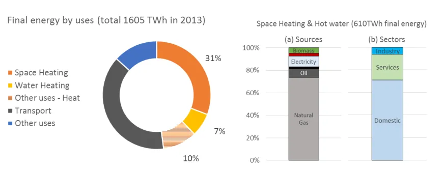
In 2013, space heating and hot water accounted for approximately 40% of total final energy 43
consumption in the UK (BEIS, 2016) and 20% of UK GHG emissions (CCC, 2016). Domestic buildings 44
were responsible for the major share of energy use for space and water heating (Figure 1). Overall, 45
space and water heating in buildings is still overwhelmingly provided by fossil fuel sources, with 46
insulation improvements can lead to some reduction in final energy use, the move to heating based 48
on heat pumps is seen as a key low-carbon heat technology by the Department for Business, Energy 49
& Industrial Strategy (BEIS) and the Committee for Climate Change (CCC) (CCC, 2015; DECC, 2011), 50
especially in buildings off the gas grid (CCC, 2016). Heat pumps can extract heat from the air, the so-51
called air source heat pump (ASHP) or the ground, the ground source heat pump (GSHP). Projected 52
numbers of new installations over the coming years are shown in Table 1, along with the actual 53
number of devices already installed in existing properties. The latest numbers for installations in the 54
UK point to a total of only 100,000 air and ground source heat pumps (CCC, 2015). The CCC estimates 55
that an additional 200,000 installations are required between 2015 and 2020 to stimulate the market 56
for heat pumps in the UK and keep on track to meeting the 2035 GHG emission budgets. 57
The GSHP has the advantage that the temperature of the ground does not vary as much as that of the 58
air, with the particular benefit that in winter, the period of maximum demand, the ground is still 59
relatively warm. In contrast, the ASHP can encounter difficulties with icing of the heat exchanger in 60
cold weather when of demand is highest though in summer the air temperature is often warmer than 61
the ground. However, the air source system is easier to install, despite potential issues with noise if 62
sited too close to neighbouring properties and buildings, hence the cost is lower. In the case of the 63
GSHP, either boreholes or ground loops are needed unless, exceptionally, a body of water is available. 64
Boreholes are expensive and access is required for the specialist equipment. Trenching for ground 65
loops (‘slinkies’) is in principle straightforward but requires a large ground area and is disruptive. 66
These factors no doubt explain why relatively large numbers of ASHPs have been installed despite the 67
existence of substantial subsidies (the renewable heat incentive (RHI)) (BEIS, 2017b; Ofgem, 2017). 68
Further issues relate to the design and operation of heat pump installations. General practice in the 69
UK has been to heat with gas, or to some extent oil, fired boilers (Figure 1). Installers are familiar with 70
these devices and sizing proceeds from guidelines based on the floor area of the property and the type 71
adequate heat output on cold (-5°C in England) days with the expectation that the heating will be on 73
for a relatively short period in the morning and a longer time in the evening so there will be high 74
transient demands. Combined with installers’ natural desire to avoid customer complaints about 75
being cold, this process leads to boilers of high rating, multiples of actual demand for much of the time 76
(Bennett et al., 2016; The Energy Saving Trust, 2009). 77
The extra cost of a larger gas or oil boiler is not great and indeed the cost of the boiler is not a dominant 78
element in the cost of a whole heating system (up to 25% of total cost of the system). In contrast, 79
heat pumps are expensive and there is therefore a strong incentive to not to oversize the system, 80
especially for GSHPs where an increase in output requires additional ground loops or boreholes. The 81
use therefore of heat pumps poses linked challenges for installers and users. From a user perspective, 82
mixed experiences have been reported, both anecdotally and in the literature (Boait et al., 2011; 83
Energy Saving Trust, 2011; 2013; DECC, 2013). Individuals used to the rapid warm-up characteristic of 84
gas fired systems may find the slow response of a heat pump based system frustrating; others have 85
bemoaned the lack of controllability and have resorted to temperature management by opening 86
windows to release excess heat (Boait et al., 2011; Liu, Shukla, & Zhang, 2014). Many of these issues 87
stem from the design of the system, reflecting installers’ lack of understanding and experience, and 88
the intrinsic limitations of some heat pumps. 89
There are also definite views on the type of property suited to heat pumps systems (Jenkins et al. 90
2009; Fawcett, 2011; Arteconi et al., 2013; Judson et al., 2015; Ali et al., 2016). It is widely asserted 91
that they are only appropriate for very well insulated, typically new build, houses with underfloor (low 92
temperature) heating. Whilst there is no doubt that these building are well suited, if there is to be a 93
significant move to heat pump based heating systems, as hoped for by BEIS and CCC, then a wider 94
range of building types must be considered. In fact, the largest CO2 savings are likely to come from
95
applying heat pumps to houses off the gas grid which are currently heated by oil (CCC, 2016; Gupta 96
gas heating, there have been no significant extensions to the gas network in recent years and it is 98
unlikely that there will be in future. Houses in this category often have quite high heating loads so the 99
CO2 savings will be considerable and often have the land required for the installation of ground loops
100
or boreholes; exceptional cases include Castle Howard where heat is extracted from a lake (MBS, 101
2011). 102
This paper investigates the practicalities of heat pump installation in older houses currently heated by 103
oil. The work is based on a case study of a former Vicarage in Cambridgeshire. The study began by 104
building a detailed thermal model for the house and verifying this against experimental measurements 105
taken from sensors in every room. The expected heating demands were then computed from the 106
model based on weather data and the GSHP was designed accordingly. The system was then installed 107
and initial operational data are presented. 108
In the longer term, there is an interest in seeing what coefficient of performance is achievable as 109
reports suggest that this deteriorates with time (Banks, 2008; Underwood, 2014), principally as a 110
permanent depression of ground develops (this is not an issue for ASHPs). It may also be that 111
[image:6.595.70.488.554.683.2]manufacturers quote optimistic and possible unrealistic performance data for their heat pumps. 112
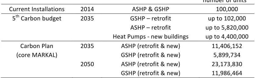
Table 1 – Current and projected heat-pump installations in existing (retrofit) and new buildings 113
under different future UK energy system scenarios (sources: CCC, 2015; BEIS, 2016; DECC, 2011) 114
number of units Current Installations 2014 ASHP & GSHP 100,000
5th Carbon budget 2035 GSHP – retrofit up to 102,000
ASHP – retrofit up to 5,820,000 Heat Pumps - new buildings up to 4,400,000 Carbon Plan 2035 ASHP (retrofit & new) 11,406,152 (core MARKAL) GSHP (retrofit & new) 5,899,734
116
Figure 1 – Space heating statistics 2013 – sectors and fuel use (based on data from (BEIS, 2016)). 117
2 The building
118
The property chosen for the study is a former vicarage, a type of building often described as ‘un-119
heatable’. The building is representative of a medium sized country house, the floor area being 120
approximately 3000 sq. ft or 300 m². There are an estimated 700,000 similar properties heated mostly 121
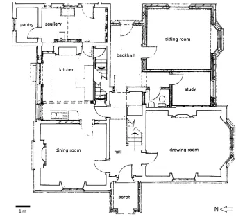
by oil with high potential CO2 savings (CCC, 2017). The ground floor plan of the house is shown in
122
Figure 2. The original building, constructed between 1871 and 1872, is of mixed construction – the 123
front part is of solid triple brick (13 1/2”/ 343 mm) and the rear part is solid 9” (229 mm) brick. For 124
uncertain reasons the house was never completed as originally designed so the present owners built, 125
more or less to the original plan, a new section in 2000-2001. The construction here was cavity wall, 126
with an outer skin of brick (4 ½”/ 114 mm), 100 mm of Rockwool insulation and an inner skin of 100 127
mm blockwork. 128
The roof over the original parts of the house is of the collar type. It was only possible to install 50 mm 129
of semi-rigid Rockwool over the sloping parts of the ceilings because of limited space whereas 200 130
mm of blanket was placed over the flat surfaces. In the new build part, the first floor ceilings all have 131
200 mm of Rockwool, the thickness required at the time of construction. The glazing is variable – in 132
the new build with two exceptions sealed double glazed units were employed. In the older part there 133
some simple single glazed windows. The ground floors are mostly insulated with 100 mm of Rockwool 135
or fibreglass but there is a small area of uninsulated solid floor in the scullery and pantry. Some 136
measures have been taken to reduce draughts but there are four open fires, three having a register 137
plate or a closer, and a stove. A cellar under the kitchen is a further source of air flow via the cellar 138
steps. The elements are summarized in Table A-1 in the Appendix. Note that although the 139
terminology used by ESP-r may differ from the actual materials in the building; the values used in the 140
modelling are SAP values for the actual elements. 141
[image:8.595.119.459.271.593.2]142
Figure 2 – Ground floor plan 143
3 Initial planning and building characterization
144
As part of the planning for the installation of the GSHP, the oil consumption from the time of the 145
completion of the 2001 building works was examined. The data show that the oil consumption for 146
performance, as shown in Figure 3. Annual usage was approximately 5000 l, noting that this figure 148
includes use by an oil burning Aga, estimated to be around 2000 l. The space heating input over the 149
year is about 32 MWh, allowing for 2 MWh for hot water. This calculation assumes the calorific value 150
of oil to be 10.35 kWh/l and the boiler’s combustion efficiency to be 80% (the manufacturer’s declared 151
efficiency for the oil boiler is 84.6%) and the Aga’s combustion efficiency in the heating period to be 152
55% (from SAP). 153
154
[image:9.595.85.484.291.484.2]155
Figure 3 – Total oil consumption for heating and hot water from 2001-2014. 156
Also as part of the planning, the installer calculated, using standard methodology (SAP), the expected 157
heating and hot water demands and found these to be 52 and 3 MWh, respectively, substantially 158
greater than the actual figure. Some adjustments, primarily allowing for the heat output from the 159
Aga, were made to the calculations to produce a figure (32 MWh) that more reasonably aligned with 160
actual consumption. It is the case that one of the bedrooms with the poorest thermal properties is 161
not heated but on the other hand the heating periods are considerably longer than normal, in 162
particular continuous heating throughout the night. As part of the application for the Renewable Heat 163
Efficiency Rating was E41, with a rating of F32 for environmental impact. The estimated heated 165
requirement was 52 MWh over a year, again higher than the actual heating requirements, even with 166
an additional 3 MWh for water heating. Understanding the reasons for the significant differences was 167
a driving factor in building a detailed thermal model of the house, both to enable a more accurate 168
sizing of the heat pump and to understand the origin of the why the SAP method leads to such an 169
overestimate. 170
As further preparatory work, temperature and humidity sensors were placed in all rooms and in the 171
attic spaces, all wireless connected to a data hub with an internet connection. Readings of 172
temperature, accurate to ±1°C are taken every 30 minutes. The heating regime, during the working 173
days, was 4.30 pm to 8.30 am the following day and was continuous at weekends. All radiators have 174
thermostatically controlled valves As an example of performance, Figure 4 shows temperatures of 175
the dining room, the bedroom over and the kitchen, the latter containing the Aga, for a day in March 176
2015. The attic temperature is a proxy for the outside temperature, which fluctuates between 6 and 177
10°C. The stability of the internal temperatures during the heating period are evident, as is the decay 178
of temperature in the bedroom and dining room once the heating is stopped. A fall in temperature 179
occurs in the kitchen, despite the presence of the Aga, suggesting a significant degree of thermal 180
182
Figure 4 - Room temperatures over a 24 hour period on 3rd – 4th of March 2015 (from temperature 183
logging). 184
The long thermal time constants evident, of the order of 24 hours or longer, are not unsurprising as 185
the construction of the house is relatively massive, with almost all internal walls being of 9” brickwork. 186
The high thermal mass combined with moderate values of thermal conductivity leads to long time 187
constants. Experiments were made to extract time constants by shutting off the radiators in a room 188
and dissipating a known power from an electric heater until an equilibrium temperature was obtained 189
followed by cooling. A fitting algorithm was then used to obtain time constants but there was 190
considerable variability in the results and the time constants for heating and cooling could be quite 191
different. One obvious problem is that for best results the outside temperature has to be nearly 192
constant, a condition only obtained on overcast winter days. In addition, rooms are thermally coupled, 193
complicating behaviour. Overall, this is an area where experimental techniques need to be developed, 194
probably in conjunction with sophisticated thermal models. 195
Recognizing that the temperature of the water for the central heating from a heat pump would have 196
autumn 2015 to its lowest value, producing an exit temperature of about 55°C but with a peak of 198
about 60°C just before the burner shuts off. 199
Although the radiator thermostatic valves have a constant setting, there is a clear temperature droop 200
and recovery. As the heat loss increases with falling outside temperature, there has to be an ever 201
greater difference between the set and actual temperatures to increase the output from the radiators. 202
This difference is exacerbated by lower circulating water temperatures; in control terms the gain of 203
the feedback loop is proportional to the difference between room temperature and circulating water 204
temperature so the smaller the difference the bigger the temperature error. Whilst a slump of 3°C is 205
not large in absolute terms, it is significant in terms of human comfort and in addition the cooler 206
outside walls will reduce the perceived temperature (which takes into account radiation) even further. 207
Several important conclusions were drawn from the initial investigations. It was reassuring to know 208
that the heating system could function in terms of an adequate heat output with a circulating water 209
temperature in the range achievable with a heat pump. Temperature control with thermostatic valves 210
would, however, be less precise. This could be overcome by electrically actuated valves but the extent 211
of cabling to implement this measure is a drawback although there are now battery operated TRVs. 212
There is the option of manual advance of settings in critical areas, notably bedrooms and bathrooms; 213
the living areas have supplementary heating anyway. A further option is making the circulating water 214
temperature dependent on the outside temperature (possible with the GSHP) to give a feed-forward 215
effect though the achievable degree of compensation was not certain. 216
The manner of operating the system is also a consideration. In fact the long thermal time constants 217
of the building lend themselves to heating with a heat pump; the expectation is that the interior of 218
the building will be maintained at essentially a steady temperature. It is accepted that the house will 219
take a considerable time to heat up from cold, or indeed change temperature rapidly. In other words, 220
4 Thermal model, including verification
222
Thermal modelling was performed with the ESP-r software package (William, 2015). The complex 223
model encompassed 29 zones, 16 of which refer to home divisions, 4 to halls and passageways, 224
another 4 to separate sections of the roof, 1 to the underfloor volume, 1 to the cellar, and 3 to the 225
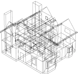
fireplaces and respective chimneys. It was initially built as closely as possible to reflect the geometry 226
and indoor areas (Figure 5), materials and constructions (Table A-1) and infiltration rates previously 227
gathered and used for the SAP evaluation. 228
The model was further refined using the sensors’ temperature measurements for each room and 229
calibrated, particularly in terms of air infiltrations and air exchange rates between rooms, with the 230
experimental data collected during the determination of time-constants. Heating periods, set-points 231
and space occupation were modelled according to actual conditions. The AGA stove in the kitchen, 232
operating continuously, was included in the model as a constant heat source of 1.37 kW during the 233
heating season (note that during the project the AGA was converted to electrical heating so actual 234
electricity consumption measurements became available) and then slightly lower over the summer 235
months, due to the lower temperature differential with the kitchen’s air temperature. 236
The closest ESP-r weather data included in ESP-r is for London, which is itself based off Gatwick airport 237
data, about 75 miles south of the building location. Cambridge University’s Digital Technology Group, 238
however, located just over 4 miles away, have compiled an archive of weather data since 1995 which 239
is freely available online (DTG, 2016). Using this data, Gatwick’s ESP-r data file was modified to account 240
for Cambridge’s conditions in the years from 2009 to 2015, thus creating one file for each of those 6 241
years. This meant replacing dry-bulb temperatures, humidity and dew-point temperatures by the 242
measurements done by the Cambridge University’s meteorological station. Given the absence of local 243
solar radiation measurements, Gatwick’s data were used instead. This is a source of error that must 244
be kept in mind when comparing the model performance with the data from the temperature and 245
247
Figure 5 – Screenshot of the model (in ESP-r) 248
The weather file also has information about monthly ground temperatures at multiple depths, but 249
these are only relevant for exposed soil. Soil temperature below the house and in contact with the 250
cellar has had the time to settle at a generally higher temperature. To adjust for this discrepancy, the 251
monthly ground temperature profiles were iteratively calibrated in such a way that modelled 252
temperatures in the cellar (almost fully underground) closely tracked the corresponding sensor 253
temperature readings. 254
Given the lack of information for local wind speeds and direction around the building, constant yearly 255
average infiltration rates were used instead, in accordance to the SAP methodology (one air-change 256
per hour for most rooms and two air-changes per hour for bathrooms and kitchen). Continuous air 257
exchanges between rooms were set at 20% to 50% of the infiltration rates taking into consideration 258
typical door opening periods. As with the solar radiation data, the lack of wind and infiltration rate 259
During the heating season, running from mid-October to mid-April, the space heating system is 261
typically turned on between 4:30pm and 8:30am on workdays and continuously over the weekends. 262
This is considered the current usage scenario. Three other heating scenarios were also tested: 263
continuous (running 24 hours per day), shorter (more closely tracking occupation periods in different
264
rooms), and setback (similar to the shorter pattern but keeping the heating system on at a lower 265
temperature of 16°C instead of completely turning it off with the aim of reducing energy 266
consumption). Figure 6 shows the schedules for each of the tested scenarios. Depending on the 267
spaces’ real usage and on the building’s thermal characteristics, different scenarios might perform 268
better or worse, be it from an energy expenditure perspective, from a comfort perspective or even 269
from a system’s dimensioning perspective. Given that the main purpose of the modelling exercise was 270
to size the heat pump system more precisely, it was very relevant to explore these different usage 271
patterns. For instance, in principle, heating for shorter periods may result in lower energy expenditure 272
but generally might require higher power requirements. 273
274
0 … … … 23 0 … … 23
Gf rooms Halls 1f rooms WC Gf rooms Halls 1f rooms WC Gf rooms Halls 1f rooms WC Gf rooms Halls 1f rooms WC
0 … … … 23 0 … … 23
Weekdays Saturdays & Sundays
Day type Schedule
Schedule Day type
22 6 7 8 22
6 7 8 16 17
16°C 22°C 16°C 22°C
16°C
16°C 19°C
19°C 16°C 19°C
16°C 22°C 16°C 22°C
16°C 19°C 16°C 19°C
19°C 16°C 19°C
21°C
Off Off
16°C 21°C 16°C 21°C 21°C
22°C 19°C 22°C 19°C 19°C Off Off Off 22°C 21°C 19°C 19°C 22°C 19°C 19°C 21°C Off Off Off Off Off Off Off 22°C 22°C 19°C 19°C 21°C 19°C 21°C 21°C 19°C 19°C 22 Cu rr en t Con tin uou s
Weekdays Saturdays & Sundays
6 7 8 16 17 22
22°C 19°C 19°C Sh or t Sh or t Se tb ac k
Figure 6– Heating system operating periods and temperature set-points for different rooms, according 275
to the four different patterns explored, i.e. current usage, continuous heating, shorter heating periods, 276
and shorter heating periods with a setback temperature of 16°C. (Gf – ground floor; 1f – 1st floor).
277
The main aim of the modelling exercise was to get a better estimate for heat required to keep the 278
building within comfortable conditions, tracking the real-world sensor temperatures as well as the 279
hourly heat flux and maximum aggregate hourly heating power. Since the model assumes simple heat 280
injection into each space, the results are independent of any particular heating equipment, but the 281
maximum heat flux in each room was limited according to the characteristics of the existing radiators. 282
These were determined during the SAP and range from 3.5 kW in the largest space (drawing room), 283
to 1 kW in the smaller rooms. 284
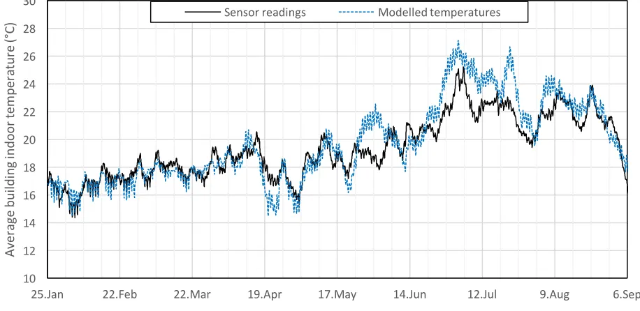
Comparing the calibrated model running in the current scenario with the real-world sensor 285
measurements, room temperatures are tracked fairly satisfactorily, albeit not perfectly (Figure 7). The 286
testing period ran from 25th of January 2015 (when sensor readings started) to the 6th of September
287
2015 (when the testing period ended). This encompasses approximately 12 weeks of conditioned 288
operation (until the 15th of April) after which the building’s heating system is turned off and the model
289
operates in free-float mode. Within this period average temperature differences between model and 290
sensor readings for each room were generally within ±1°C, with standard deviations ranging from 291
approximately 1°C in the halls and kitchen, to close to 2°C in rooms with less predictable usage and 292
heating patterns, such as, for example the drawing room (the log-burning stove in the fireplace is used 293
sporadically). 294
In some instances, differences of up to ±6°C were seen between real-world sensors and model results. 295
There are a number of aspects that keep the model from better tracking the real-world temperatures, 296
namely: unpredictable user operation of doors, windows, curtains and shutters was either ignored or 297
integrated in simplified ways (e.g. closing shutters at night and opening during the day, regardless of 298
real conditions); the sporadic use of fireplaces, cooking, and other heat-releasing equipment was not 299
wind speed measurements and building air permeability were absent, thus building ventilation was 301
simplified to constant airflows according to SAP recommended values; the model does not account 302
for the impacts of any indoor furniture. The impact of these aspects can be clearly seen in the 303
comparison of indoor temperatures shown in Figure 7. For instance, during the hottest period, around 304
July, frequent window and door opening and extensive building ventilation resulted in significantly 305
lower indoor temperatures than the ones predicted by the model. During the conditioned period, 306
where the simulation more closely follows real building operation, model temperatures track the 307
sensor readings significantly better. 308
Despite the less than perfect tracking, for the purpose of more precise sizing of the heat pump 309
equipment, these results were considered to provide a good balance between calibration effort and 310
accuracy of simulation. While it is clear that dynamic building simulation would provide much better 311
estimates of the heating demand of the building than simpler methodologies, and in particular SAP, it 312
is also recognized that the estimates can never be perfect. At some point, the effort required in further 313
refining and calibrating the model would outweigh the usefulness of the added precision. 314
[image:17.595.73.531.473.696.2]315
Figure 7 – Comparison between sensor readings and modelled whole building average indoor 316
temperatures for the testing period (from 25th January to the 6th of September of 2015)
317
10 12 14 16 18 20 22 24 26 28 30
25.Jan 22.Feb 22.Mar 19.Apr 17.May 14.Jun 12.Jul 9.Aug 6.Sep
Av
er
ag
e
bu
ild
in
g
in
do
or
te
m
pe
ra
tu
re
(°
Between 2009 and 2015, 2010 was the coldest year in Cambridge. For that year the model estimates 318
annual heating needs at 31.5 MWh while using the current heating pattern (Table 2). Those needs 319
change to 34.3 MWh, 23.9 MWh and 26.9 MWh if heating continuously, for shorter periods or using a 320
setback temperature set-point instead of turning the system off, respectively. However, for 2014 the
321
estimates are approximately 30% lower, as a clear demonstration of the impact that weather can have 322
in energy requirements for space heating. These results exclude the AGA output, which contributes 323
around 9 MWh over the year. 324
Table 2 - Estimated yearly heating needs (in MWh) for the warmest and coldest years since 2009 (i.e. 325
2014 and 2010, respectively) and according to different heating patterns. 326
Heating pattern
Year Current Continuous Shorter Setback
2010 31.5 34.3 23.9 26.9
2014 23.0 25.2 17.2 18.7
327
Considering the worst case scenario, i.e. continuous heating during the coldest year (34.3 MWh), the 328
space heating needs calculated through thermal modelling still end up being approximately 1/3 lower 329
than the SAP calculation of 51.7 MWh/annum. Discrepancies between the SAP calculations and real-330
world energy needs, especially for buildings built pre-1900, are well known and the results here 331
presented seem to corroborate this (Laurent et al., 2013; Gupta and Irving, 2013; Summerfield et al., 332
2015; Gupta and Gregg., 2016). In particular, it presents an argument against using SAP estimates for 333
sizing heating systems. 334
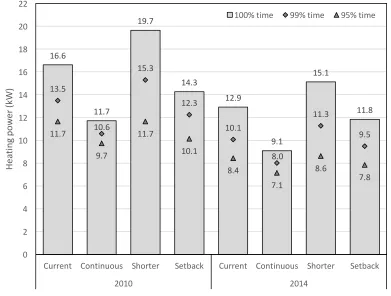
The modelled space heating power requirements traced for different years and heating patterns 335
should be a better strategy for correctly sizing new heating systems and avoiding oversizing. Figure 8 336
shows the power requirements for 2014 and 2010, the warmest and coldest years since 2009 in 337
Cambridge, and for different heating patterns. Without changing the current heating pattern, the 338
highest estimated power output required to meet the heat demand all of the time is just over 16.5 339
only 95% of the time, then 12 kW should be enough. This would mean failing to meet demand for 341
approximately 55 hours in 2010 (but only 5 hours in 2014). Since most of these hours occur right after 342
the system is turned on, the issue would manifest itself in indoor temperatures taking somewhat 343
longer to reach comfortable levels. 344
As shown previously, the current heating pattern turns off the heating system during the middle of 345
the weekdays (from 8:30 to 16:30), when residents are off for work. When the system is turned on at 346
the end of the afternoon, the estimated power demand tends to be higher, since the building has been 347
cooling down for 8 hours. If, instead, the space is continuously heated, power requirements for 348
meeting demand 95% of the time are reduced to just over 10 kW. Conversely, operating the heating 349
system in shorter bursts would get power requirements up to close to 20 kW for meeting demand all 350
the time. Interestingly, whilst an extra 5 kW in heating power is required to supply the final 5% of 351
demand in the current heating pattern, only a further 2 kW is required if heating continuously. An 352
354
Figure 8 – Estimated heating power requirements needed to cover 100% (bars), 99% (diamonds) and 355
95% (triangles) of the time space heating is required. Showing the results for 2014 and 2010 (warmest 356
and coldest year since 2009, respectively) and for the tested space heating patterns. 357
358
These results also show that there is a balance to be established between energy saving and 359
equipment power requirements. While the shorter heating pattern saves the most energy (about 25% 360
compared to current), it requires a significantly more powerful system for meeting the last 5% of 361
heating demand (up to 18% more). The opposite is found when running the system continuously, 362
requiring the lowest system power (approximately 20%) while demanding the highest total energy 363
expenditure (9% higher than current). A good balance appears to be achieved by using the setback
364
strategy, which simultaneously requires lower power (roughly 10%) and saves energy (about 15%) 365
when compared to turning off the system completely during the middle of weekdays as in the current
366
pattern. These results favour a judicious adjustment of heating schedules as a way to optimizing the 367
use of appropriately sized heat pump systems. 368
5 GSHP system design and installation
369 16.6 11.7 19.7 14.3 12.9 9.1 15.1 11.8 13.5 10.6 15.3 12.3 10.1 8.0 11.3 9.5 11.7 9.7 11.7 10.1 8.4 7.1 8.6 7.8 0 2 4 6 8 10 12 14 16 18 20 22
Current Continuous Shorter Setback Current Continuous Shorter Setback
2010 2014 He at in g po w er (k W )
The starting point was the choice of heat pump. During the planning of the project a modulating heat 370
pump came on to the market, manufactured by Mastertherm, with an approximately 3:1 output 371
range. This device appeared attractive as for much of the heating period the actual heating demand 372
is quite modest, with peak demand occurring for only a relatively few days. It is desirable to limit the 373
cycling of heat pumps and this is usually achieved by a suitably sized buffer tank. If the heat pump can 374
reduce its output then the size of buffer tank can be reduced. From the thermal modelling, a capacity 375
of 16 kW would have sufficed for all recent years except the coldest (2010) when it would have been 376
inadequate for just 5 hours. 377
Whilst Masterthem produces a 16 kW pump, the preferred supply is three-phase and the house only 378
has a single phase supply, albeit with a 100 A rating, noting that the house at one point had electric 379
storage heaters. A quotation was obtained from the local Distribution Network Operator for a three-380
phase connection but the cost was prohibitive; it would have added about 40% to the project cost. 381
Therefore the 12 kW heat pump was chosen, recognizing that this would ‘brown out’ for several days 382
each winter (e.g. 218 hours in 2010), to see how tightly the rating could be specified. As a result 383
supplementary heating would be needed either by boosting the output of the heat pump with its 384
integral electrical heater or by the use of an existing log-burning stove or open fires or even free-385
standing electric heaters. The occasional inconvenience was considered acceptable. 386
The worst case for heat pump cycling can be shown to be at half its minimum output. In the case of 387
the chosen model, this is 4 kW so to keep starts to three per hour for a change in water temperature 388
of 5°C with a heating load of 2 kW, a tank capacity of 114 l is needed. As there is a considerable volume 389
of water in the primary circuit pipework, a 100 l tank was specified. For heating loads above 4 kW, 390
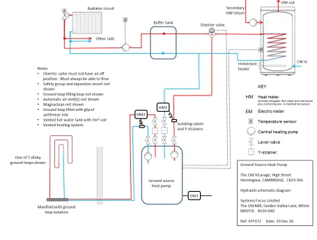
392
Figure 9 – GSHP system diagram. 393
Overall control is by the existing programmer which has separate control of hot water and heating. 394
When the heating is active, the heat pump circulates primary water through the buffer tank; for this 395
to happen the diverter valve must be energized. Water is circulated through the radiators by a 396
separate pump irrespective of circulation from the heat pump. The heat pump will act to maintain 397
the primary circulation within a target temperature range, either by modulating its output or by 398
shutting off for periods. The target temperature range can be set to reflect the outdoor temperature 399
determined by a separate sensor. 400
Domestic hot water has priority. A temperature sensor in the domestic hot water cylinder signals to 401
the heat pump if heat is needed. If heating is active, the diverter valve is de-energized, transferring 402
the required cylinder temperature is reached, noting that the target temperature for this is 404
independently set. There is provision for a sterilization cycle involving heating the hot water to 60°C. 405
The primary water temperature for the central heating will have a maximum value of 50°C. All the 406
radiators were assessed to see if they would have adequate output at this temperature. Fortunately, 407
many rooms have cast iron radiators with rated outputs specified for 60°C water temperature and 408
these turned out to be sufficiently generously sized that acceptable performance could be expected 409
at 50°C. In contrast, some rooms had steel panel radiators with rated outputs specified at 70°C water 410
temperature and not all these may be able to perform satisfactorily with the reduced water 411
temperature. It was decided to see how well they worked and replace as needed. Overall, the 412
philosophy was that in cases of inadequate output, in the first instance measures should be looked at 413
to reduce heat loss. 414
Knowing the rating of the heat pump allowed the ground loop to be specified. A cautious view of the 415
loading of the ground loops was taken partly because of a desire to avoid the risk of icing and partly 416
to allow for some increase in heat pump capacity in the future. The design called for five loops each 417
of 300 m of pipe in parallel, each circuit pre-formed by the supplier into 50 loops each using 4 m of 418
pipe and with a repeat distance of 1 m, with a 25 m tail and a 75 m return pipe. The site, although 419
having overall adequate space, was rather awkward. Three circuits could be accommodated in a lawn 420
to the west of the house and the other two in a lawn to the south but in both cases in serpentine 421
trenches which complicated excavation. 422
After discussion with the installer it was decided to place the loops in the vertical plane, minimizing 423
the overall amount of spoil. The main trenches were 2 m deep, giving nominally 800 mm of cover 424
over the apices of the coils, and 300 mm wide. The trench carrying the go and return pipes to the 425
west lawn were 1 m deep and 1 m wide to enable the go and return pipes to be separated. All pipes 426
were buried directly in earth, with care taken to avoid pressure points from sharp stones, except 427
tape was placed over pipe runs. Care was also taken not to bend the pipes around too tight a radius 429
or rest on sharp corners. The ground conditions were variable with bands of so-called lower chalk (a 430
mix of clay and chalk), sand and gravel. Some of the lower chalk was quite hard, slowing excavation. 431
In the one area the bottom of the trench was below the water table at the time of excavation which 432
could be helpful but the level of the water table does fluctuate. 433
Excavating a trench for one circuit took one to two days, with backfilling taking a similar time. Care 434
was taken to reserve top-soil to aid the restoration of the lawn and whilst this was largely achieved, 435
the serpentine structure evident in Figure 10 made excavation and backfilling difficult. During 436
backfilling there was a heavy rainstorm which caused considerable additional compaction of material; 437
it was difficult to achieve good compaction initially as the trench was narrow and deep. Subsequently 438
the trenches were flooded in turn to ensure good compaction as a ready supply of water was available 439
from an old well. The five loops were terminated in a manifold on the exterior of the house with go 440
and return pipes going through a wall to the heat pump. The loops were flushed, antifreeze 441
introduced followed by water before being de-aerated in turn using the valves on the manifold and 442
an external pump. The circuits were found to be leak tight. 443
The heat pump itself was installed on the other side of an external wall to the manifold, allowing a 444
straightforward connection (Figure 9). The ground loop was pressurized to 1.5 bar using a normal 445
pressurizing vessel as used in closed heating systems. A slow fall of pressure was noticed but this was 446
due to a small leak in one of the manifold connections – this was remedied by tightening the joint. 447
Flow meters were fitted in the ground loop and the output circuits along with temperature sensors so 448
that the heat inputs and outputs can be measured. The electrical input is also monitored, enabling 449
the coefficient of performance to be estimated but accuracy is limited by the fact that there are two 450
452
Figure 10 - Photo of ground loop excavation. 453
The installation of the buffer tank was next. Providing separate circuits for hot water and heating so 454
that the buffer tank could be adjacent to the heat pump was initially considered but this idea was 455
rejected as duplicating the existing pipe runs to the airing cupboard would mean lifting recently re-456
laid floors. The buffer tank has therefore been sited in the airing cupboard above the existing hot 457
water cylinder, accepting the drawback that the water in the pipework between the heat pump and 458
airing cupboard, containing approximately 40 l of water, could cycle in temperature and to a degree 459
compromise the efficiency of the heat pump. Reconfiguration of the pipework was also necessary; 460
the final arrangement is shown in Figure 9. 461
6 Preliminary results
462
Although the ground loops had been installed by the autumn of 2015, further design work was needed 463
on the configuration of the indoor system so the final implementation was postponed until the end of 464
the heating season in spring 2016. During the summer of 2016 the production of domestic hot water 465
was studied and it was noted that even at the minimum heat output the primary water temperature 466
rose quite rapidly whilst the secondary water was still cool with a temperature difference around 8°C 467
as the existing hot water cylinder had a heat exchanger area of 0.6 m2. A new 160 l cylinder with a 3
469
m2 heat exchanger was chosen but delivery was delayed so the new cylinder was not installed until
470
the end of the heating season in April 2017, completing the changes to the plumbing system. 471
Operational data have been recorded from December 22nd 2016, with an all-day heating regime being
472
operated until February 19th 2017 when it was changed to the reduced hours scheme, namely off
473
between 8.30 am and 4.30 pm. The heat pump’s external temperature feature was used with a linear 474
variation in the temperature of water supplied for heating between break-points of 30°C at 15°C 475
external temperature and 47.5°C at -5°C outside temperature. The heat delivered to the house was 476
measured using a Vuheat grade 2 heat meter and the electrical input was recorded using a standard 477
kWh meter. Over the all-day heating period 2626 kWh of electricity were consumed and 7691 kWh 478
delivered as heat, giving a ratio of heat to electrical input of 2.93. The lowest return temperature to 479
the ground loop observed was 1 °C. 480
Daily thermal output rose to about 170 kWh during periods of below freezing outside temperatures 481
but interior temperatures were maintained at around 18 °C. Under these conditions the average heat 482
output of just over 7 kW meant that the demanded output was within the heat pump’s modulation 483
range so operation was continuous. The average interior temperature over the period was 18.8°C, 484
excluding Bedrooms 3 and 4 and the scullery which were not heated. The heat pump was also 485
providing domestic hot water requiring an estimated 320 kWh based on an annual demand of 2 MWh. 486
However, the Aga contributed 1940 kWh and some use, particularly in the evenings, was made of the 487
wood burning stove in the drawing room (30 occasions) and the open fire in the dining room (18 488
occasions); the heat contribution is estimated to be 250 kWh. Making these adjustments gives a 489
heating input of 9561 kWh for the period. 490
Modelling was performed to determine the expected consumption over the period in question, 491
adjusting operation to mimic the real conditions. This meant using continuous heating, turning off 492
and other adjacent spaces (i.e. assuming that doors were kept close most of the time), and removing 494
the heat input on the scullery that was previously a result of heat losses in the oil boiler and exposed 495
piping network. The modelled result of 9328 kWh for the period is in good agreement with the real-496
world heating contribution from the heat pump. This includes a modelled AGA contribution of 1973 497
kWh but does not take into consideration the needs for heating the domestic hot water. 498
Based on these results, if oil had been burnt to generate 7.69 MWh of heat with a calorific value of 499
10.35 kWh/l and a CO2 intensity of 3.18 kg/l, and assuming a boiler efficiency of 0.85, 2.78 t of CO2
500
would have been released. The electricity used, assuming a CO2 intensity of electricity consumption
501
of around 305 g/kWh2, involved the release of 800 kg of the gas, a saving of 1.97 t. Over a year the
502
predicted saving is approximately 7 t and this saving will increase as the production of electricity is 503
decarbonized. 504
7 Discussion and conclusion
505
Results to date support the initial proposition that, with careful design, a GSHP based system can 506
replace an oil boiler and thereby lead to substantial savings of CO2 in the type of property considered.
507
Key to the design has been the detailed thermal modelling which provided the confidence to use a 508
heat pump with a modest rating which reduces costs in important areas such as the construction of 509
the ground loop array, the heat pump itself and possible increasing the capacity of the electricity 510
supply as the installed cost worked out at approximately £2,000/kW. The significant differences 511
between the modelling undertaken for this project in terms of predicted heating needs, which tallies 512
with actual previous experience, and the standard assessment procedure is a matter of concern as the 513
latter leads to significant oversizing of plant. From an RHI perspective it also leads to higher payments 514
2 Average CO
2 intensity for electricity consumed over period from 1st of December 2016 to 1st of March 2017, as
calculated from electricinsights.co.uk (Drax, 2017), following the methodology presented in (Stafell, 2017). As a guide, BEIS estimates average 220gCO2 per kWh of electricity produced for whole of 2016 (BEIS, 2017a), which
to householders, as these are on a deemed basis related to the expected heating needs, though this 515
will not be unwelcome to householders. Clearly there is much to be gained by good thermal modelling 516
but achieving this may not be realistic unless persistent weaknesses in the SAP approach can be 517
identified and corrected. Historic fuel consumption records are another way of building confidence. 518
The project was financially attractive although the installation, especially of the ground loops, was 519
disruptive. The project cost was just over £20,000 and the RHI was initially £5491 per annum but this 520
is indexed. Expected annual electricity consumption is expected to cost about £1200 so, even making 521
allowances for maintenance, the payback time will be five to seven years. 522
User behaviour and expectations are important in a successful project. In the present case, radiators 523
with thermostatically controlled valves were retained so relatively good temperature control of 524
individual rooms was achieved, notwithstanding the increased degree of temperature droop. In this 525
regard the heating system has familiar characteristics but on the other hand if the blast of heat first 526
thing in the morning is an important part of the user’s experience then the system will be a 527
disappointment. Significant night time setback is impossible anyway given the thermal time constants 528
involved so a cooler night-time temperature is not practical. In the present house this is circumvented 529
by a separate dressing room. All parties had extensive discussions about what was expected and trials 530
in advance of the project established the acceptability of the proposed mode of operation. 531
Good support from the installer was very valuable. Unusually the installation company was led by a 532
Chartered Engineer which facilitated discussions on the basis of engineering principles as opposed to 533
simply trade experience. The subtlety of system design can be beyond the knowledge of an electrician 534
or plumber even if they have attended specialist courses which are no substitute for degree-level 535
understanding. 536
The installation of the ground loops was successful but it is clear that it is much easier to deal with one 537
straight trench per circuit both in terms of excavation and manipulation of the slinky assembly. A heat 538
is not so much of an issue in larger houses. The modifications to the plumbing arrangements can be 540
awkward though in this case a lot of time invested in design of a suitable layout made it possible to 541
make the changes in under two days, minimizing the time without hot water. Electrical 542
reconfiguration was somewhat tedious as the heat pump takes in low voltage control signals whereas 543
as conventional heating controls work at mains voltage so it was necessary to make a custom relay 544
box. Finally, as noted in what is believed to be the first domestic heat pump installation (Haldane, 545
1930), there is the question of noise and vibration. In the present installation the heat pump is sited 546
in an extremity of the house so noise from the heat pump itself not an issue but some vibration is 547
being transmitted through the fixings for the primary pipework. Means of mitigating this are being 548
investigated. 549
Long term monitoring of the project is underway to track the co-efficient of performance of the heat 550
pump, to determine if there is a significant depression of ground temperature around the ground 551
loops, to see if the overall heat output is adequate for most days, to see if the any upgrading of 552
radiators is needed and to assess the quality of the user experience. The results are expected to 553
support the initial conclusion that successful GSHP installations can be made in properties that have 554
not generally been considered suitable provided that careful assessment and design work are 555
undertaken. It is the authors’ intention to publish these results in due course with full details of the 556
instrumentation used. Finally, it is not argued that conventional radiators systems are the preferred 557
choice for use with heat pumps, rather that there are many older properties of the type considered in 558
this study where the installation of say underfloor heating is not practical in terms of cost, structural 559
limitations or simply a preference for traditional suspended wooden floors. In the British Isles alone 560
there are potentially around 700,000 of off-gas grid solid wall homes in similar conditions (CCC, 2017) 561
and there are more in regions with a similar climate and building traditions e.g. northern France where 562
oil accounts for 16% of the total energy for heating in residential buildings (Ministère de la Transition 563
écologique et solidaire, 2015). To exclude these properties would forego a substantial step towards 564
Acknowledgements
566
The authors wish to thank Bruce Burnett of Systemsfocus Ltd., an MCS registered installer, for 567
generous assistance during the project. Zenaida Sobral Mourao’s research is funded by ESPRC through 568
the Whole System Energy Modelling (wholeSEM) consortium, EPSRC Grant number EP/K039326/1. 569
Hugo Santos gratefully acknowledges the funding of Project NORTE-01-0145-FEDER-000010 – Health, 570
Comfort and Energy in the Built Environment (HEBE), cofinanced by Programa Operacional Regional 571
do Norte (NORTE2020), through Fundo Europeu de Desenvolvimento Regional (FEDER). 572
573
References
574
Ali, A., Mohamed, M., Abdel-Aal, M., Schellart, A., & Tait, S. (2016). Analysis of ground-source heat 575
pumps in north-of-England homes. Proceedings of the Institution of Civil Engineers - Energy, 1– 576
13. http://doi.org/10.1680/jener.15.00022. 577
Arteconi, A., Hewitt, N. J., Polonara, F. (2013). Domestic demand-side management (DSM): Role of 578
heat pumps and thermal energy storage (TES) systems. Applied Thermal Engineering, 51 (1–2), 579
155-165. http://dx.doi.org/10.1016/j.applthermaleng.2012.09.023. 580
BEIS. (2016). Energy Consumption in the UK (2016). Retrieved from 581
https://www.gov.uk/government/uploads/system/uploads/attachment_data/file/541163/ECU 582
K_2016.pdf 583
BEIS. (2017a). 2015 UK Greenhouse gas emissions, final figures. Retrieved from 584
www.gov.uk/government/uploads/system/uploads/attachment_data/file/589825/2015_Final_ 585
Emissions_statistics.pdf. 586
BEIS. (2017b). RHI deployment data: January 2017. Retrieved from 587
Bennett, G., Elwell, C., Lowe, R., & Oreszczyn, T. (2016). The Importance of Heating System Transient 589
Response in Domestic Energy Labelling. Buildings, 6(3), 29. 590
http://doi.org/10.3390/buildings6030029 591
Boait, P. J., Fan, D., & Stafford, A. (2011). Performance and control of domestic ground-source heat 592
pumps in retrofit installations. Energy and Buildings, 43(8), 1968–1976. 593
http://doi.org/10.1016/j.enbuild.2011.04.003 594
CCC. (2015). Sectoral scenarios for the Fifth Carbon Budget. Retrieved from 595
https://www.theccc.org.uk/wp-content/uploads/2015/11/Sectoral-scenarios-for-the-fifth-596
carbon-budget-Committee-on-Climate-Change.pdf 597
CCC. (2016). Next Steps for UK heat policy. Retrieved from https://www.theccc.org.uk/wp-598
content/uploads/2016/10/Next-steps-for-UK-heat-policy-Committee-on-Climate-Change-599
October-2016.pdf 600
CCC. (2017). Annex 2. Heat in UK buildings today. Retrieved from https://www.theccc.org.uk/wp-601
content/uploads/2017/01/Annex-2-Heat-in-UK-Buildings-Today-Committee-on-Climate-602
Change-October-2016.pdf 603
DECC. (2011). The Carbon Plan: Delivering our low carbon future. Retrieved from 604
https://www.gov.uk/government/uploads/system/uploads/attachment_data/file/47613/3702-605
the-carbon-plan-delivering-our-low-carbon-future.pdf 606
DECC. (2013). Analysis from the Energy Saving Trust’s heat pump field trial, Retrieved from: 607
https://www.gov.uk/government/publications/analysis-from-the-first-phase-of-the-energy-608
saving-trust-s-heat-pump-field-trial 609
DEFRA. (2015). UK’s Carbon Footprint 1997-2013. Retrieved from 610
Drax (2017). Drax Group Ltd. Electric Insights. Accessed on the 14th of July 2017. URL:
612
https://electricinsights.co.uk
613
DTG. (2015). Digital Technology Group University of Cambridge - Cambridge Weather. Retrieved 614
from https://www.cl.cam.ac.uk/research/dtg/weather/ 615
Energy Saving Trust (2009). Final Report: In-situ monitoring of efficiencies of condensing boilers and 616
use of secondary heating. Prepared by Gastec at CRE Ltd for the Energy Saving Trust. Retrieved 617
from: www.gov.uk/government/uploads/system/uploads/attachment_data/file/180950/In-618
situ_monitoring_of_condensing_boilers_final_report.pdf 619
Energy Saving Trust. (2010). Getting warmer: a field trial of heat pumps. Retrieved from: 620
www.energysavingtrust.org.uk/Media/node_1422/Getting-warmer-a-field-trial-of-heat-pumps-621
PDF 622
Energy Saving Trust. (2013). The heat is on: heat pump field trials phase 2. Retrieved from: 623
www.energysavingtrust.org.uk/Media/node_1422/Getting-warmer-a-field-trial-of-heat-pumps-624
PDF 625
Fawcett T. (2011). The future role of heat pumps in the domestic sector. In: Proceedings of the ECEEE 626
2011 Summer Study, Energy Efficiency First : the foundation of a low-carbon society. The 627
European Council for an Energy Efficient Economy (ECEEE). 628
Gupta, R., Irving, R. (2014). Possible effects of future domestic heat pump installations on the UK 629
energy supply. Energy and Buildings, 84, 94-110. 630
http://dx.doi.org/10.1016/j.enbuild.2014.07.076. 631
Gupta, R., & Gregg, M. (2016). Do deep low carbon domestic retrofits actually work? Energy and
632
Buildings, 129, 330–343. http://doi.org/10.1016/j.enbuild.2016.08.010
633
electricity. IEEE, 68 (402), 666–675. 635
Hannon, M. J.. (2015). Raising the temperature of the UK heat pump market: Learning lessons from 636
Finland. Energy Policy, 85, 369-375. http://dx.doi.org/10.1016/j.enpol.2015.06.016. 637
HM Government. Climate Change Act 2008 (c27), The Stationery Office Ltd, London 1–103 (2008). 638
HM Government. Retrieved from 639
http://www.legislation.gov.uk/ukpga/2008/27/pdfs/ukpga_20080027_en.pdf 640
Jenkins, D.P., Tucker, R., Rawlings, R. (2009). Modelling the carbon-saving performance of domestic 641
ground-source heat pumps. Energy and Buildings, 41, 587–595. 642
http://dx.doi.org/10.1016/j.enbuild.2008.12.002 643
Judson, E. P. and Bell, S., Bulkeley, H., Powells, G. and Lyon, S. M. (2015). The co-construction of 644
energy provision and everyday practice: integrating heat pumps in social housing in England. 645
Science and technology studies, 28 (3).
646
Kelly, J. A., Fu, M., Clinch, J. P. (2016). Residential home heating: The potential for air source heat 647
pump technologies as an alternative to solid and liquid fuels. Energy Policy, 98, 431-442. 648
http://dx.doi.org/10.1016/j.enpol.2016.09.016. 649
Laurent, M.-H., Allibe, B., Tigchelaar, C., Oreszczyn, T., & Hamilton, I. (2013). Back to reality : How 650
domestic energy efficiency policies in four European countries can be improved by using 651
empirical data instead of normative calculation. Eceee Summer Study Proceedings., 2057–2070. 652
Retrieved from http://discovery.ucl.ac.uk/1403583/ 653
Liu, S., Shukla, A., & Zhang, Y. (2014). Investigations on the integration and acceptability of GSHP in 654
the UK dwellings. Building and Environment, 82, 442–449. 655
http://doi.org/10.1016/j.buildenv.2014.09.020 656
ménages en 2012. Chiffres & statistiques, 645. Retrieved from: 658
http://www.statistiques.developpement-659
durable.gouv.fr/publications/p/2348/1041/consommations-energetiques-menages-2012.html 660
Modern Building Services (MBS) (2011). 661
http://www.modbs.co.uk/news/archivestory.php/aid/9524/Stately_homes_exploit_water__fe 662
atures_for_heat_pumps.html 663
Ofgem. (2017). Tariffs and payments: Domestic RHI | Ofgem. Retrieved from 664
https://www.ofgem.gov.uk/environmental-programmes/domestic-rhi/contacts-guidance-and-665
resources/tariffs-and-payments-domestic-rhi/current-future-tariffs 666
Staffell, I. (2017). Measuring the progress and impacts of decarbonising British electricity, Energy
667
Policy, 102, 463-475; doi: 10.1016/j.enpol.2016.12.037.
668
Underwood, C. (2014). On the Design and Response of Domestic Ground-Source Heat Pumps in the 669
UK. Energies, 7(7), 4532-4553; doi:10.3390/en7074532.
670
William, J. (2015). Strategies for Deploying Virtual Representations of the Built Environment (aka The 671
ESP-r Cookbook). Retrieved from http://www.esru.strath.ac.uk/Documents/ESP-672
r_cookbook_june_2015.pdf 673
674
675
Appendix
676Details of elements and their thermal properties 677
Construction U-Value
(W/m².K) Elements/materials Thickness (mm) Therm. cond. (W/m.K) Original 13.5'' external
brick wall 1.561 Brick (UK code) Dense plaster 12.5 343 0.77 0.50 Original 9'' external brick
wall 2.031 Brick (UK code) Dense plaster 12.5 229 0.77 0.50 Insulated original 9''
external brick wall (used in the kitchen)
0.895 Brick (UK code) 229 0.77
Glasswool (generic) 25 0.04
Dense plaster 12.5 0.50
Recent external insulated brick wall
0.286 Brick (UK code) 114 0.77
Fiberglass batt insulation 100 0.036 Vermiculite insulating brick 100 0.27
Dense plaster 12.5 0.5
Original 9'' internal brick
wall 1.933 Dense plaster Brick (UK code) 12.5 229 0.77 0.5
Dense plaster 12.5 0.50
Internal partition cavity
brick wall 0.884 Dense plaster Vermiculite insulating brick 12.5 100 0.50 0.27
Air gap/cavity 50 0.14
Vermiculite insulating brick 100 0.27
Dense plaster 12.5 0.50
Internal partition wall 1.930 Plasterboard (UK code) 12.7 0.21
Breeze block 100 0.44
Plasterboard (UK code) 12.7 0.21
Roof 6.346 Clay tile 6 0.85
Roofing felt 2 0.19
Roof on 1st floor sloping
ceiling sections 0.686 Clay tile Roofing felt 6 2 0.85 0.19
Glasswool (generic) 50 0.04
Dense plaster 25.4 0.50
1st floor ceiling (20 cm
insulation) 0.185 Hardboard (standard density) Glasswool (generic) 200 25 0.13 0.04 Plasterboard (UK code) 12.7 0.21 Ground floor ceiling 1.548 Wilton weave wool carpet 5 0.06 Hardboard (standard density) 25 0.13
Air gap/cavity 75 0.14
Plasterboard (UK code) 12.7 0.21 Ground flooring (with 10
cm insulation)
0.328 Wilton weave wool carpet 5 0.06 Hardboard (standard density) 25 0.13
Glasswool (generic) 100 0.04
Plasterboard (UK code) 13 0.21 Ground flooring (with 5
cm insulation) 0.572 Wilton weave wool carpet Hardboard (standard density) 25 2 0.06 0.13
Glasswool (generic) 50 0.04