To appear inOptimization
Vol. 00, No. 00, Month 20XX, 1–28
Primal and Dual Algorithms for Optimisation over the Efficient Set
Zhengliang Liua∗and Matthias Ehrgottb
aSchool of Electronic Engineering and Computer Science, Queen Mary University of London, London E1 4NS, United Kingdom
bDepartment of Management Science, Lancaster University Management School, Bailrigg, Lancaster LA1 4YX, United Kingdom
(Received 00 Month 20XX; accepted 00 Month 20XX)
Optimisation over the efficient set of a multi-objective optimisation problem is a mathematical model for the problem of selecting a most preferred solution that arises in multiple criteria decision making to account for trade-offs between objectives within the set of efficient solutions. In this paper we consider a particular case of this problem, namely that of optimising a linear function over the image of the efficient set in objective space of a convex multi-objective optimisation problem. We present both primal and dual algorithms for this task. The algorithms are based on recent algorithms for solving convex multi-objective optimisation problems in objective space with suitable modifications to exploit specific properties of the problem of optimisation over the efficient set. We first present the algorithms for the case that the underlying problem is a multi-objective linear programme. We then extend them to be able to solve problems with an underlying convex multi-objective optimisation problem. We compare the new algorithms with several state of the art algorithms from the literature on a set of randomly generated instances to demonstrate that they are considerably faster than the competitors.
Keywords:Multi-objective optimisation, optimisation over the efficient set, objective space algorithm, duality.
1. Introduction
Multi-objective optimisation deals with optimisation problems with multiple conflicting objectives. It has many applications in practice, e.g. minimising cost versus minimising adverse environmental impacts in infrastructure projects [13], minimising risk versus maximising return in financial portfolio management [23] or maximising tumour control versus minimising normal tissue complications in radiotherapy treatment design [11]. Because a feasible solution simultaneously optimising all of the objectives does not usually exist, the goal of multi-objective optimisation is to identify a set of so-called efficient solutions. Efficient solutions have the property that it is not possible to improve any of the objectives without deteriorating at least one of the others. In practical applications of multi-objective optimisation it is generally necessary for a decision maker to select one solution from the efficient set for implementation. This selection process can be modelled as the optimisation of a function over the efficient set of the underlying multi-objective optimisation problem. For example, an investor may aim at minimising the transaction cost of establishing a portfolio with high return and low risk. If such a function that describes the decision maker’s preferences is explicitly available, one might expect that it is computationally easier to directly optimise the function over the efficient set rather than to solve the multi-objective optimisation problem first and then obtain a most preferred
∗
efficient solution – in particular because the efficient set can in general be an infinite set (see Figures 1 and 2 below). Secondly, decision makers may be overwhelmed by the large size of the whole efficient set and may not be able to choose a preferred solution from it in a very effective manner. These considerations have motivated research on the subject of optimisation over the efficient set since the 1970s.
We contribute to this research with new algorithms and new results on how to identify optimal solutions of this problem. In Section 2 we provide the mathematical preliminaries on multi-objective optimisation and necessary notation. A revised version of Benson’s outer approximation algorithm and its dual variant are summarised in Section 3. In Section 4, we survey algorithms for optimisation over the efficient set from the literature. As a new contribution, we identify a subset of the vertices of the feasible set in objective space at which an optimal solution must be attained. Based on the outer approximation algorithm we then propose a new primal algorithm in the all linear case by incorporating a bounding procedure in the primal algorithm of [18] in Section 5. Furthermore, this primal algorithm is extended to maximise a linear function over the non-dominated set of a convex multi-objective optimisation problem. Section 6 proposes a new dual algorithm for optimisation over the non-dominated set, which makes use of a new result providing a geometrical interpretation of optimisation over the non-dominated set. This dual algorithm is also further developed to maximise a linear function over the non-dominated set of a convex problem. The numerical experiments in Section 7 compare the performance of our new primal and dual algorithms with algorithms from the literature that we discuss in Section 4. The results reveal that our algorithms, in particular the dual algorithm in the linear case, are much faster (up to about 10 times) than comparable algorithms from the literature.
2. Preliminaries
A multi-objective optimisation problem (MOP) can be written as
min{f(x):x ∈ X}, (1)
where f : Rn → Rp is a function, which we assume to be continuous, and X is a feasible set in decision space Rn. LetY := {f(x) : x ∈ X} denote the image of X in objective space Rp. We assume that X is a nonempty and compact set. Therefore, Y is nonempty and compact, too. The feasible setY in objective space is bounded by the vectors of componentwise minima and maxima denoted byyI andyAI, respectively, i.e., ykI 5 yk 5 ykAI for all y ∈ Y. These two points are called the ideal and anti-ideal point, respectively.
We use the following notation to compare vectors y1,y2 ∈ Rp: y1 < y2if y1k < yk2for
k = 1, . . . ,p; y1 5 y2 if y1k is componentwise less than or equal to y2k and y1 ≤ y2 if y1 5 y2but y1 , y2. We also defineRp
= := {y ∈ R
p
:y = 0}andRp≥ := {y ∈ Rp :y ≥ 0}=Rp=\ {0}. SetsRp5,Rp≤andR
p
< are defined analogously.
Definition 1 A feasible solutionxˆ ∈ Xis called a (weakly) efficient solution of (1)if there
is no x ∈ X such that f(x) ≤ (<)f(xˆ). The set of all (weakly) efficient solutions is called the (weakly) efficient set in decision space and is denoted by X(W)E. Correspondingly,
ˆ
y = f(xˆ)is called a (weakly) non-dominated point andY(W)N := {f(x): x ∈ X(W)E}is the (weakly) non-dominated set in objective space.
In this case, as well as ifYN =Y the optimisation problem we study in this paper becomes either trivial or becomes a standard single objective optimisation problem.
In case all objectives of (1) are linear and the feasible setXis polyhedral (1) is called a multi-objective linear programme (MOLP) and can be written as
min{C x:x ∈ X}, (2)
where C is a p×n matrix. The feasible setX is defined by linear constraints Ax = b, where A∈Rm×n andb ∈ Rm. A polyhedral convex set such asXhas a finite number of faces. A subset F ofX is a face if and only if there are ω ∈ Rn\ {0}and γ ∈ Rsuch thatX ⊆ {x ∈Rn :ωTx = γ}andF = {x ∈Rn :ωTx = γ} ∩ X. We call a hyperplane
H= {x∈Rn:ωTx =γ}supportingXatx0ifωTx = γfor allx ∈ XandωTx0=γ. The proper(r−1)-dimensional faces of anr-dimensional polyhedral setXare called facets of X. Proper faces of dimension zero are called extreme points or vertices ofX.
In Example 1 we provide a numerical example of a multi-objective linear programme, which we shall use throughout the paper.
Example1 min 1 0 0 1 x1 x2 s.t. © « 4 1 3 2 1 5 −1−1
1 0 0 1 ª ® ® ® ® ® ® ® ¬ x1 x2 = © « 4 6 5 −6 0 0 ª ® ® ® ® ® ® ® ¬
Figure 1 shows the feasible setXof Example 1 as well as its imageYin objective space (due toCbeing the identity matrix). The bold line segments compose the non-dominated setYN. Furthermore, in this exampleXE is the same asYN.
y1 y2
1 2 3 4 5 6
[image:3.595.214.369.462.629.2]1 2 3 4 5 6 0 Y a b c d e f
Figure 1. The image of the feasible set of the MOLP of Example 1 in objective space.
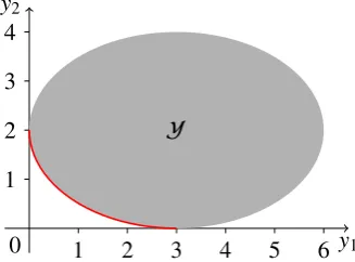
Example2
min
1 0 0 1
x1 x2
s.t.
(x1−3)2
9 +
(x2−2)2
4 5 1
.
The image of the feasible set in objective space is illustrated in Figure 2. The bold curve is the non-dominated set of the CMOP.
y1 y2
0 1 2 3 4 5 6
1 2 3 4
[image:4.595.208.372.190.311.2]Y
Figure 2. The image of the feasible set of the CMOP of Example 2 in objective space.
To solve multi-objective optimisation problems is generally understood as obtainingYN, and for each pointy ∈ YN somex ∈ XE with f(x)= y. This paper is concerned with the optimisation of a function over the efficient set of a multi-objective optimisation problem,
max {Φ(x):x ∈ XE}, (3)
whereΦ(x):Rn →Ris a function ofx.
In general, (3) is a difficult global optimisation problem [6, 17, 20, 24, 25]. This is due to the fact that the efficient set of even a multi-objective linear programme is nonconvex (see Example 1). As such, there exist local optima, which may differ from global optima. In Example 1, assumingΦ(x)= x1+x2,(0,4)T is a local optimal solution. Along the efficient edges from(0,4)T to(0.4,2.4)T and(9/13,20/13)T the objective value decreases, before increasing again to the global optimal solution at (5,0)T. Furthermore, since the feasible set of (3) is the efficient set of an MOP it can in general not be explicitly expressed in the form of a system of inequalities prior to solving the problem.
Fülöp [16] has shown the equivalence of optimisation over the efficient set to a bilevel optimisation problem and NP-hardness of the problem. In Example 3 we demonstrate that the bilevel optimisation approach even in the case of optimising a linear function over the efficient set of an MOLP does in general lead to a nonlinear optimisation problem.
Example3 Consider an all linear version of (3), i.e.,
max µTC x:x ∈ XE , (4)
whereXE is the efficient set of the MOLP
(4) and (5) can be regarded as a bilevel optimisation problem, where (4) is the upper level problem and (5) is the lower level problem. The constraint x ∈ XE in (4) can be replaced by the well known optimality conditions for MOLP, see e.g. Ehrgott [10]. Feasible solution
x ∈ Xis efficient if and only if there existλ∈R>p andu ∈Rm
= such that A
Tu =λTC and λTC x=bTu.
Therefore (4) can be rewritten as
max µTC x :Ax =b,ATu=CTλ, λTC x= bTu,u =0, λ > 0 . (6)
While (6) has a linear objective function and some linear constraints, it also has quadratic constraints and requires thatλbe strictly positive. Hence solving (6) will be considerably more difficult than solving a linear programme. Example 3 thus provides one motivation for research in algorithms to solve (3) in the linear case: is it possible to derive algorithms that only make use of linear programming techniques?
In multi-objective optimisation it is well known that, because the number of objective functions is usually much smaller than the number of decision variables, the structure of Y is most often simpler than the structure ofX. In particular, in multi-objective linear programming, the structure and properties ofXE andYN are well investigated. [9] notes that Y often has fewer extreme points and faces than X. [8] illustrates the concept of “collapsing”, which means that faces ofXshrink into nonfacial subsets ofY. [1] shows that the dimension of efficient faces in the feasible set always exceeds or equals the dimension of their images in Y. Hence, it is arguably more computationally efficient to employ techniques and methods to solve (3) in objective space, and algorithms for optimisation over the efficient set have followed this trend since 2000. The algorithms we propose in this paper fall in this category, too.
In this context, we assume that the objective functionΦof (3) is a composite function of a function M : Rp → R and the objective function f of the underlying MOP, i.e., Φ = M◦ f. Therefore,Φ(x) = M(f(x)). Substituting y = f(x) into (3), we derive the problem of optimisingMover the non-dominated setYN of an MOP:
max {M(y):y∈ YN}. (7)
Problem (7) is essentially the same problem as (3) but appears to be more intuitive than (3), because in practice decision makers typically choose a preferred solution based on the objective function values rather than the value of decision variables.
In this article, the problems we are interested in are two special cases of (7) namely (8) and (10) defined below.
max µTy:y ∈ PN , (8)
where µ ∈ Rp and PN is the non-dominated set of the upper image P := Y+Rp= of an MOLP (2). Note that the set of vertices ofP,VP ⊂ PN = YN, i.e., all vertices ofP are non-dominated, and the non-dominated sets ofY andPcoincide. Moreover,PN is a subset of the boundary of P, see for example [10], Proposition 2.4. It is easy to see that Theorem 1 holds for problem (8).
Theorem 1 There exists an optimal solutiony∗of (8)at a vertex ofP, i.e., y∗∈VP, the
set of vertices ofP.
of the upper imageY+Rp=of of a CMOP.
max µTy:y ∈ PN . (9)
Because the upper imagePof a CMOP is a convex (but not necessarily polyhedral) set, we will in general not be able to compute it or its non-dominated subset exactly. Hence we consider approximations ofPN using the concept of-non-dominance as defined below. Definition 2 Let ∈R, >0. A pointyis called (weakly)-non-dominated ify+e∈ Y,
whereeis a column vector with all elements being one, and there does not exist anyyˆ ∈ Y
such that yˆ ≤ (<)y.
Consequently we change Problem (9) by replacingPN withPN, an-non-dominated set of the upper image of a CMOP.
max µTy:y ∈ PN . (10)
3. Outer Approximation Algorithms in Multi-objective Optimisation
3.1. Multi-objective linear programming
Theorem 1 suggests that in order to solve (8) an algorithm to identify extreme points (vertices) of P is needed. Benson [2] proposed an outer approximation algorithm to compute the non-dominated setYN of an MOLP. The authors of [12] revised this method in such a way that it considers Prather thanY and in [18] it was further developed by reducing the number of LP subproblems that need to be solved (1 rather than 2 in each iteration). This revised version of Benson’s algorithm first constructs a p-dimensional polyhedron S0 := yI +Rp= such that P ⊆ S0. In every iteration it chooses a vertex si from the vertex setVSi−1 which is not inPand constructs a supporting hyperplane toP
by solving an LP and obtaining its dual variable values.Siis then defined by intersecting Si−1with the halfspace of the supporting hyperplane containingPand updating the vertex set of Si. The algorithm terminates as soon as no suchsi ∈ Si−1\ P can be found and thereforeSi =P. At termination both a vertex and an inequality representation ofPare known. [12] propose a dual variant of Benson’s algorithm to solve (13), which has been further developed by [18].
We first provide notation that will facilitate the description of the subsequent algorithms. Fory ∈Rpandv ∈Rp, let
λ(v):= v1, ...,vp−1,1− p−1
Õ
i=1 vi
!T
, (11)
λ∗
(y):= y1−yp, ...,yp−1−yp,−1
T .
(12)
Consider the weighted sum scalarisationP1(v)of (2)
Proposition 1 Letv ∈Rp≥such that
Íp
k=1vk 51.Then an optimal solutionxˆto(P1(v))
is a weakly efficient solution to the MOLP(2). The dualD1(v)ofP1(v)is
max bTu:u∈Rm,u =0,ATu=CTλ(v) . (D1(v)) Given a point y ∈ Rp in objective space, the following LP (P2(y)) serves to check the feasibility of y, i.e., if the optimal value ˆz > 0, theny is infeasible, otherwisey ∈ P. An optimal solution(xˆ,zˆ) ∈ X ×Rto (P2(y)) provides a weakly non-dominated point ˆy =Cxˆ ofP.
min{z:(x,z) ∈Rn×R,Ax= b,C x−ez 5 y}. (P2(y)) The following LP (D2(y)) is the dual of (P2(y)).
max bTu−yTλ:(u, λ) ∈Rm×Rp,(u, λ) =0,ATu=CTλ,eTλ=1 . (D2(y)) Proposition 2 is the key result for the revised version of Benson’s algorithm.
Proposition 2 [18] Let(u∗, λ∗)be an optimal solution to (D2(y)). Then p
Õ
k=1 λ∗
kyk =b Tu∗
is a supporting hyperplane toP.
Therefore, by solving(P2(y)), we not only check the feasibility of pointybut also obtain the dual variable values (u∗, λ∗) as optimal solutions to (D2(y)) by which we construct a supporting hyperplane toP.
[19] introduced a concept of geometric duality for multi-objective linear programming. This theory relates an MOLP with a dual multi-objective linear programme in dual ob-jective spaceRp.In dual objective space, we use the following notation to compare two vectors v1,v2 ∈ Rp. We write v1 >K v2 if vk1 = vk2 for k = 1, . . . ,p−1 andv1p > v2p; v1 =
K v2ifvk1= vk2fork =1, . . . ,p−1andv1p = vp2. Moreoverv1 ≥K v2is the same as v1>K v2.
The dual of MOLP is
max K
(λ1, ..., λp−1,b Tu)T
:(u, λ)= 0,ATu=CTλ,eTλ=1 , (13)
where (u, λ) ∈ Rm × Rp. K := {v ∈ Rp : v1 = v2 = · · · = vp−1 = 0,vp = 0} is the ordering cone in the dual objective space, and maximisation is with re-spect to the order defined by K. Let V denote the feasible set in the dual objec-tive space, then its lower image is D := V − K. The K-maximal set of D is DK=
v∈ V :v=maxK {(λ1, ..., λp−1,b Tu)T
:(u, λ) =0,ATu=CTλ,eTλ=1} . Fig-ure 3 shows the lower image D in the dual objective space of Example 1. The bold line segments composeDK.
In [19] two set-valued mapsHandH∗are defined to relatePandD.
0 1 D
[image:8.595.217.365.49.203.2]v1 v2
Figure 3. Lower image of (13) for the MOLP of Example 1.
H*:Rp ⇒Rp,H*(y):=v ∈Rp :λ∗(y)Tv =−yp . (15)
Given a point v ∈ Rp in dual objective space H(v) defines a hyperplane in primal objective space. Similarly, given a point y ∈ Rp in primal objective space H∗(y) is a hyperplane in dual objective space.Theorems 2 and 3 state a relationship between proper K-maximal faces ofD and proper weakly non-dominated faces ofP.
Theorem 2 [19]
(1) A point v is a K-maximal vertex of D if and only if H(v) ∩ P is a weakly non-dominated facet ofP.
(2) A pointyis a is a weakly non-dominated vertex of Pif and only ifH∗(y) ∩ Dis a
K-maximal facet ofD.
[19] define a duality mapΨ: 2R
p
→2Rp
. LetF∗ ⊂Rp, then
Ψ(F∗):= Ù v∈ F∗
H(v) ∩ P.
Theorem 3 [19]Ψis an inclusion reversing one-to-one map between the set of all proper K-maximal faces ofDand the set of all proper weakly non-dominated faces ofPand the inverse map is given by
Ψ−1(F )= Ù y∈ F
H∗(y) ∩ D.
Moreover, for every properK-maximal faceF∗ofDit holds thatdimF∗+dimΨ(F∗)=
p−1.
Therefore, given a non-dominated extreme pointyex ∈ P, the correspondingK-maximal facet ofDisH∗(yex) ∩ D.
3.2. Multi-objective convex optimisation
We review an extension of Benson’s outer approximation algorithm proposed by [22]. It provides a set of-non-dominated points by means of approximating the non-dominated set of a convex MOP. Similar to the revised version of Benson’s algorithm for computingPNin the case of an MOLP this algorithm iteratively constructs a polyhedral outer approximation of the upper imagePof a CMOP. It starts with a polyhedronS0= yI+Rp=containingP. In each iterationi, a vertex ofSi−1that is not an-non-dominated point ofPis randomly chosen to generate a supporting hyperplane to P. Then the approximating polyhedron is updated by intersecting it with the half-space containing P defined by the supporting hyperplane. The algorithm terminates when all of the vertices ofSiare-non-dominated with a vertex and inequality representation of polyhedronSicontainingP.
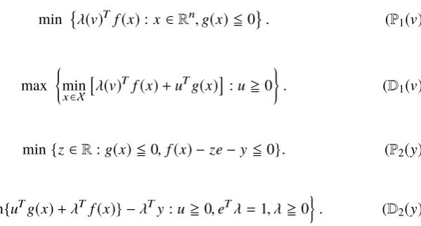
We introduce two pairs of single objective optimisation problems to facilitate the de-scription of algorithms later. Problem P1(v) is a weighted sum problem. Solving P1(v) results in a weakly non-dominated point. ProblemD1(v)is the Lagrangian dual ofP1(v). Because we work with Lagrangian duals, we will from now on assume that the functions defining the MOP are differentiable. ProblemsP2(y)andD2(y)are employed to generate supporting hyperplanes. These four optimisation problems are the nonlinear extensions of the LPsP1(v),D1(v),P2(y)andD2(y), respectively. They involve nonlinear convex terms making them harder to solve than their LP counterparts.
min λ(v)T f(x):x ∈Rn,g(x) 50 . (P1(v))
max
min x∈X
λ(
v)T f(x)+uTg(x)
:u=0
. (D1(v))
min {z∈R:g(x)5 0, f(x) −ze−y 5 0}. (P2(y))
max
n
min x {u
Tg(x)+λT f(x)} −λTy
:u= 0,eTλ=1, λ=0
o
. (D2(y))
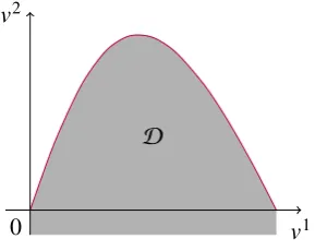
The outer approximation algorithm of [22] for convex MOPs approximates the non-polyhedral P (see Example 2) generating a set of -non-dominated points. Löhne et al. [22] propose a dual variant of the convex version of Benson’s algorithm (see Section 5.3). The geometric dual of a convex MOP is defined as
max
K {D(v):v ∈R
p, λ(v) ≥
0}, (16)
where D(v) = v1, . . . ,vp−1,minx∈X
λ(
v)Tf(x)
. The ordering cone K := {v ∈ Rp : v1=v2 =· · ·=vp−1=0,vp = 0}is the same as in (13), and maximisation is with respect to the order defined byK. LetVdenote the feasible set in the dual objective space, then its lower image in the dual objective space isD :=V − K. TheK-maximal set of (16) is
DK =max K
(λ1, ..., λp−1,min x∈X
λ(v)T
f(x))T :(u, λ)= 0,eTλ=1
[image:9.595.181.481.323.484.2].
K-maximal set. This is modelled by the concept ofK-maximum, which is defined in Definition 3.
Definition 3 Let ∈Rand >0. A pointvis called anK-maximal point ifv−ep ∈ D
and there does not exist anyvˆ ∈ Dsuch thatvjˆ =vjforj =1, . . . ,p−1andvpˆ >vp.
D
v1 v2
[image:10.595.219.364.142.257.2]0
Figure 4. The lower image of the CMOP of Example 2 in dual objective space.
The dual version of the convex Benson algorithm for solving CMOPs performs an outer approximation to D. This algorithm first chooses an interior point in D. This is implemented in the way stated in Algorithm 2, Step i1 in [12]. Then a polyhedron S0 containing D is constructed. In each iteration a vertex si of Si−1 that does not belong to DK is chosen. By solving (P1(si)), a supporting hyperplane to D is determined. Eventually, a set of K-maximal points of D is obtained, the convex hull of which extended by−K is an outer approximation polyhedron ofD.
4. A Review of Algorithms for Optimisation over the Efficient Set
In the literature there are two main categories of algorithms for optimisation over the effi-cient set: Algorithms based on decision space methods and algorithms based on objective space methods. The former approaches search for optimal solutions in decision space, whereas the latter ones explore the non-dominated set in objective space. In this section, we review some algorithms of the latter class, to which our new algorithms are compared in computational experiments. A more comprehensive review of the literature up to 2001 can be found in [25].
4.1. Bi-objective branch and bound algorithm
In this section we describe a bi-objective branch and bound algorithm to solve a special case of (7), whereM(y)is a lower semi-continuous function on the non-dominated set of a bi-objective linear programming problem. The bi-objective linear programming problem possesses some special properties, which help exploit the structure of the problem. This method was first proposed by Benson and Lee [4] and further improved by Fülöp and Muu [17].
Let m1 = min {y1 : y2 = y2I,y ∈ Y}, and m2 = min {y2 : y1 = y1I, y ∈ Y}. Let y1 = (yI
1,m2) T
max M(y):(y22−y12)y1+(y11−y12)y2= y11y22−y12y12,y ∈ Y . (17) In the objective space, (17) means to find an optimal point over the region bounded by the non-dominated set and the line connectingy1andy2. Having solved problem (17), we have found an upper bound. In the case that M(y) is nonlinear, branching steps may now take place. Let the line segment connectingy1andy2shift parallel until it becomes a supporting hyperplane to Y at some pointq. By connecting both y1 and y2 with q, the branching process splits the problem into two subproblems. For each of the subproblems the same process is repeated until the upper bound and the lower bound coincide. Computational experiments can be found in [17].
In [21] this method is extended to maximise an increasing function M(y)over the non-dominated set of a convex bi-objective optimisation problem. The first step is to determine y1 and y2 and a lower bound in the same way as the linear version by [17]. These two points and the ideal point yI define a simplex. The objective functionM(y)is maximised over the intersection ofYand the simplex so that an upper bound on the optimal objective function value can be attained. A pointqat the intersection of a ray emanating from the origin and Y is determined. Pointq splits the simplex into two, each of which is to be explored in the subsequent iterations. The simplices with upper bounds that are worse than the incumbent objective function values are pruned. This process is iterated until the gap between the upper bound and the lower bound is within a tolerance determined initially by the decision maker.
4.2. Conical branch and bound algorithm
Another branch and bound algorithm was proposed in [24] to optimise a continuous function over the non-dominated set of an MOP. A conical partition technique is employed as the branching process. ConeyAI−R=pwith vertexyAIis constructed. This cone contains Y. Along each extreme direction−ekof the cone, the intersection pointykof the direction and the weakly non-dominated set PW N of the upper imageP =Y+Rp=of the MOP is obtained. If any of these points is non-dominated a lower bound is found. Then solving problem (18), a relaxation of (7), finds an upper bound.
max
(
M(y):y−Uλ= yAI, p
Õ
i=1
λi =1, λ= 0,y ∈ Y
)
, (18)
whereUis a matrix containing column vectorsyk−yAIfork =1, . . . ,p. For the branching step, a ray emanating fromyAIand passing through the centre point of the simplex spanned by the yk vectors hits the boundary ofY at a non-dominated point and a lower bound is achieved. The initial cone is partitioned. By evaluating each new cone, the gap between the upper bound and the lower bound is narrowed. A cone is called active if there is a gap between the upper bound and lower bound. An active cone will be further explored. A cone is incumbent if the upper bound meets the lower bound with the best objective value so far. A cone is fathomed if the best feasible solution found in this cone is suboptimal. An optimal point is obtained when the upper bound coincides with the lower bound.
obtained by intersecting the smaller cones with the feasible set in objective space, which provides new upper bounds. This process is repeated until the upper bound and the lower bound coincide or the gap between them is small enough.
4.3. Outcome space algorithm
A branch and bound technique also plays an essential role in the algorithm of [3]. This algorithm is designed for globally optimising a finite, convex function over the weakly ef-ficient set of a nonlinear multi-objective optimisation problem that has nonlinear objective functions and a convex, non-polyhedral feasible region. An initial simplex containingYis constructed and a branching procedure is performed. However, compared to the case where all of the constraints and objectives are linear, it is more complicated to find a feasible point and therefore to establish lower bounds. In order to find lower bounds, a subroutine is developed that requires solving several optimisation problems to detect feasible points. A relaxed problem is used to find upper bounds by using a convex combination of the vertices of the simplex. The reader is referred to [3] for more details.
5. The Primal Algorithms
5.1. Properties of optimisation over the non-dominated set of an MOLP
In this section, we investigate some properties of problem (8). It is well known that an optimal solution to (3) with linear function Φ and underlying MOLP is attained at an efficient vertex ofX, see [5]. The version of this result for problem (8), Theorem 1, implies that a naïve algorithm for solving (8) is to enumerate the vertices of P and determine which one has the largest value of µTy. This is summarised in Algorithm 1.
Algorithm 1Brute force algorithm. Input: A,b,C, µ
Output: y∗, an optimal solution to (8) Phase 1: ObtainVP.
Phase 2: y∗=argmaxµTy :y∈VP .
In Phase 1 both the revised Benson algorithm and its dual variant are capable of finding
VP. However, taking advantage of properties of (8) may dispense with the enumeration of all vertices ofP. We start this discussion by investigating the vertices ofYmore closely. Let[a−b]denote an edge of polyhedronYwith verticesaandb. We call pointsaandb neighbouring vertices and denote withN(a)the set of all neighbouring vertices of vertex
a.
Definition 4 Let[a−b]be an edge ofY.[a−b]is called a non-dominated edge if for
some pointyin the relative interior of[a−b],y ∈ YN.
According to [26] (Chapter 8) a point in the relative interior of a face of Y is non-dominated if and only if the entire face is non-non-dominated.
Definition 5 Vertexa ∈VP is called a complete vertex if all facesF ofPcontaininga
are non-dominated, otherwise it is called an incomplete vertex. LetVPc denote the set of complete vertices ofP, and defineVPic:=VP\VPc as the set of incomplete vertices.
whereaseand f are vertices ofYbut not ofP.
Proposition 3 Letabe a vertex ofY. If there does not exist a vertexb∈N(a)such that µT(b−a)>
0, thenais an optimal solution of the linear programme(19),
max µTy:y ∈ Y . (19)
Proof. Assumeais not an optimal solution, then there exists at least one vertexb∈N(a) such thatµTb> µTa, which means µT(b−a)> 0,a contradiction. Theorem 4 (19)has at least one optimal solution that is also an optimal solution to(8)
if and only ifµ∈Rp
5.
Proof. (1) Let µ ∈ Rp5. Define µ0 := −µ, then µ0 ∈ Rp= and we rewrite (19) as min{µ0TC x : x ∈ X}, which is a weighted sum scalarisation of the underlying MOLP. It is well known that there exists an efficient solution x∗ ∈ X which is an optimal solution to this problem. Therefore,y∗=C x∗∈ PN. Hence,y∗is an optimal solution to (8).
(2) Now, let µ<R5p and assume that y∗is an optimal solution to (8). Choosed ∈R≥ such thatdj =1if µj >0anddj =0otherwise. Lety0= y∗+dand >0. Since P=Y+Rp=,y0 ∈ Yfor sufficiently small. However,µTy0 = µTy∗+ µTd > µTy∗ and so y∗is not an optimal solution to (19).
Using similar arguments as in the proof of Theorem 4 it is in fact possible to show that µ∈Rp<if and only if the set of optimal solutions of both (8) and (19) is identical.
Proposition 4 Let µ ∈ Rp \R5p. If y ∈ VPc, then there exists y
0 ∈
N(y) such that
µT(y0−y)> 0.
Proof. Let µ and y be as in the proposition. If there were no y0 ∈ N(y) such that µT(y0−y) >
0, then by Proposition 3,ywould be an optimal solution to (19). Asyis also a non-dominated point, y would be an optimal solution to (8). According to Theorem 4
this implies µ∈R5p, a contradiction.
The main result of this section is Theorem 5.
Theorem 5 For all µ∈Rp\R5p there exists an optimal solutiony∗of (8)inVPic∩VP,
i.e. at an incomplete non-dominated vertex.
Theorem 5 also explains why optimising over the non-dominated set of a bi-objective linear programme is easy. In the case p = 2 the extreme points of P can be ordered according to increasing values of one objective and therefore decreasing order of the other objective. It follows thatYhas exactly two incomplete non-dominated extreme points (in Figure 1 these are a and d). These two extreme points are the non-dominated extreme points obtained by lexicographically optimising the objectives in the order (1,2) and (2,1) respectively. Hence forp=2objectives, (8) can be solved by linear programming, solving two lexicographic LPs or four single objective LPs.
5.2. The primal algorithm for solving(8)
Algorithm 1 has two distinct phases, vertex generation and vertex evaluation. Combining both phases and exploiting the results of Section 5.1 we expect that we can save computa-tional effort, since not all vertices of Pneed to be enumerated. More specifically, once a new hyperplane is generated and added to the inequality representation ofP, a set of new extreme points of the outer approximating polyhedronSiis found. EvaluatingµTyat these extreme points, we select the one with the best function value assi+1in the next iteration. If the selected point is infeasible, we proceed with adding a cuty∈Rp:Ípk=1λkyk = bTu as in the revised version of Benson’s algorithm. We call this an improvement cut. Other-wise we have a feasible solution to (8) and therefore a lower bound on its optimal value and we add what we call a threshold cut. A threshold cut is{y ∈Rp: µTy = µTyˆ}, where
ˆ
y is the incumbent solution, i.e., the best feasible non-dominated point found so far. A threshold cut removes the region where points are worse than ˆy. This primal method is detailed in Algorithm 2.
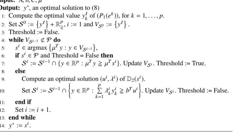
Algorithm 2Primal algorithm for solving (8). Input: A,b,C, µ
Output: y∗,an optimal solution to (8)
1: Compute the optimal valueykIof(P1(ek)), fork =1, . . . ,p. 2: SetS0 := yI +R=p,i:=1andVS0:=
yI .
3: Threshold := False. 4: whileVSi−11 Pdo
5: si ∈argmaxµTy :y ∈VSi−1 ,
6: ifsi ∈ Pand Threshold = Falsethen
7: Si :=Si−1∩ {y ∈Rp :µTy = µTsi}. UpdateVSi. Threshold := True.
8: else
9: Compute an optimal solution(ui, λi)ofD2(si). 10: SetSi :=Si−1∩
y ∈Rp : p
Í
k=1 λi
ky i k = b
Tui
. UpdateVSi. Threshold := False.
11: end if 12: Seti:=i+1. 13: end while 14: y∗:=si.
Y
y1 y2
1 2 3 4 5 6 1
2 3 4 5 6
0
S0
y1 y2
1 2 3 4 5 6 1
2 3 4 5 6
0
S1
y1 y2
1 2 3 4 5 6 1
2 3 4 5 6
0
S2
y1 y2
1 2 3 4 5 6 1
2 3 4 5 6
0
S3
y1 y2
1 2 3 4 5 6 1
2 3 4 5 6
0
[image:15.595.104.476.47.304.2]S4
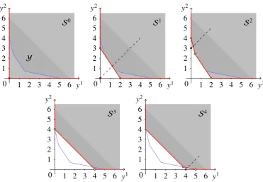
Figure 5. Iterations of the primal algorithm 2 in Example 4.
Table 1. Iterations of the primal algorithm 2 in Example 4.
i Vertexsi Cut type Candidates Non-dominated points µTy
1 (0,0) Improvement (2,0),(0,3) ∅ 3
2 (0,3) Improvement (2,0) (0,4), (0.4,2.4) 4
3 (0,4) Threshold (4,0) (0,4) 4
4 (4,0) Improvement ∅ (0,4), (5,0), (3.75,0.25) 5
Figure 5 and Table 1 show in each iteration the extreme point chosen, the type of cut added and the incumbent objective function value. In the first iteration, an improvement cut is added generating two new vertices,(2,0)T and(0,3)T. Then(0,3)T is chosen in the next iteration because it provides the best objective function value so far. The second iteration improves the function value to 4. Since(0,4)T is feasible, a threshold cut,y1+y2 =4, is then added. Although it does not improve the objective function value, this cut generates a new infeasible vertex(4,0)T. An optimal point,(5,0)T, is found after another improvement cut has been generated.
5.3. The primal algorithm for solving(10)
A naïve algorithm for (approximately) solving (10) is to obtain a set of-non-dominated points ofP(vertices ofSi) through the algorithm of [22] and to determine which one has the largest value of µTy, in the same way as in Algorithm 1.
incumbent solution. A threshold cut removes the region where points are worse than ˆy. At the end of the algorithm, an -non-dominated point y∗is obtained, which is an optimal solution to (10). Furthermore, By solving(P2(y∗)), we can find an element ˆyofPN, which is an approximate solution to (9). We also know that y∗ 5 yˆ 5 y∗+e, where is the approximation error predetermined by the decision maker. As a result, we have solved (10) exactly and determined an approximate solution ˆyto (9). This primal algorithm is detailed in Algorithm 3.
Algorithm 3Primal algorithm for solving (10). Input: f,g, µ,
Output: y∗, an optimal solution to (10) and ˆy, an approximately optimal solution to (9) 1: Compute the optimal valueykIof(P1(ek)), fork =1, . . . ,p.
2: SetS0 := yI +R=pandi:=1. 3: Threshold = False.
4: whileVSi−11 PN do
5: si ∈argmaxµTy :y ∈VSi−1 .
6: ifsi ∈ PN and if Threshold = Falsethen
7: Si :=Si−1∩y∈Rp:µTy = µTsi . Threshold := True. 8: else
9: Compute an optimal solution(ui, λi)ofD2(si). 10: SetSi :=Si−1∩
y ∈Rp :
p
Í
k=1 λi
ky i k = b
Tui
. Threshold = False. UpdateVSi.
11: end if 12: Seti:=i+1. 13: end while
14: y∗∈argmaxµTy:y ∈VSi−1 .
15: Find an optimal solution ˆx toP2(y∗). An approximately optimal solution to (10) is ˆ
y = f(xˆ).
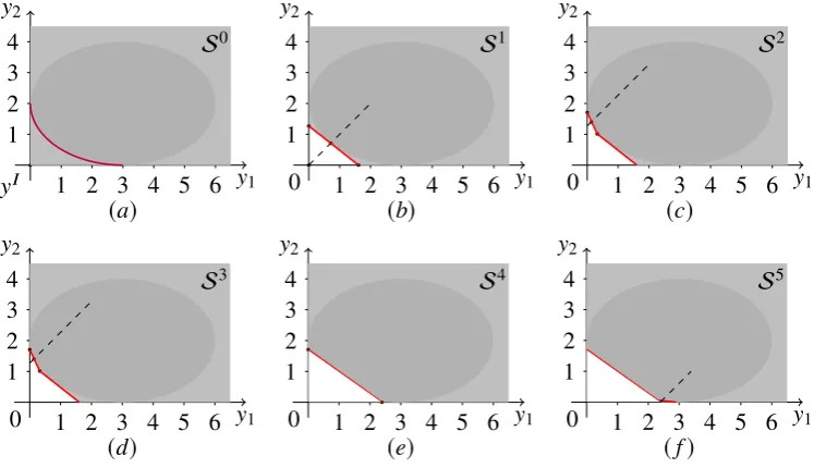
Example 5 We illustrate Algorithm 3 through maximising 5y1 + 7y2 over the non-dominated set of the CMOP of Example 2.
y1 y2
yI 1 2 3 4 5 6 1
2 3
4 S0
(a)
y1 y2
0 1 2 3 4 5 6 1
2 3
4 S1
(b)
y1 y2
0 1 2 3 4 5 6 1
2 3
4 S2
(c)
y1 y2
0 1 2 3 4 5 6 1
2 3
4 S3
(d)
y1 y2
0 1 2 3 4 5 6 1
2 3
4 S4
(e)
y1 y2
0 1 2 3 4 5 6 1
2 3
4 S5
[image:16.595.104.478.484.699.2](f)
Table 2. Iterations of Algorithm 3 in Example 5.
i Vertexsi Cut type Candidates -non-dominated points µTy
1 (0,0) Improvement (0,1.27),(1.61,0) ∅ 8.88
2 (0,1.27) Improvement (1.61,0) (0.32,1.01), (0,1.71) 11.94
3 (0,1.71) Threshold (2.39,0) (0,1.71) 11.94
4 (2.39,0) Improvement ∅ (2.9,0), (2.3,0.06) 14.51
Figure 6 and Table 2 show the iterations of Algorithm 3. In the first iteration, an improvement cut is added generating two new vertices, (0,1.27)T and (1.61,0)T. Then (0,1.27)T
is chosen in the next iteration because it provides the best objective function value so far. The second iteration improves the function value to 11.94. Since(0,1.71)T is -non-dominated, a threshold cut, 5y1+7y2= 11.94, is then added. Although it does not improve the objective function value, this cut generates a new infeasible vertex(2.39,0)T. An-non-dominated pointy∗=(2.9,0)T, is found after another improvement cut has been generated. By solvingP2(y∗)we obtain an approximately optimal solution(2.9001,0.001)T and objective function value 14.5075.
6. The Dual Algorithms
In this section, we introduce dual algorithms to solve (8) and (10) in dual objective space. The dual algorithms are derived from dual variants of Benson’s algorithm [18, 22]. We commence the discussion with some properties of (8) in dual objective space. We then introduce the dual algorithms for solving (8) and (10).
6.1. The dual algorithm for solving(8)
In this section, we explore some properties of (8) in dual objective space, which enable us to solve (8) more efficiently than by the primal algorithm of Section 5. We call the resulting algorithm the dual algorithm.
Let yex be an extreme point of P. Hence yex ∈ YN. Via set-valued map H∗, yex corresponds to a hyperplaneH∗(yex)in the dual objective space,
H∗(yex)=v ∈Rp:λ∗(yex)Tv =−yexp ,
=nv ∈Rp:(yex 1 −y
ex
p )v1+, ...,+(y ex p−1−y
ex
p )vp−1−vp =−yexp
o
.
Moreover, µandyex define a hyperplaneHye x in primal objective space
Hye x =y ∈Rp: µTy = µTyex . (20)
We notice that without loss of generality we can assume that µ ≥ 0. Otherwise we set ˆ
µk =−µkand ˆyk =−yk wheneverµk <0and ˆµk = µk and ˆyk = yk wheneverµk = 0to rewrite (20) as
Hyˆe x =yˆ ∈Rp: ˆµTyˆ = µˆTyˆex . (21)
Let us now define µ0 := Íip=1µiand divide both sides of the equation in (21) by µ0to obtain
Hye x =
ˆ
y ∈Rp : µˆ T
ˆ y µ0 =
ˆ µT
ˆ yex µ0
Since (22) is a hyperplane in the primal objective space, it corresponds to a pointvµin dual objective space. According to geometric duality theory, in particular (12), this point is nothing but
vµ =
µ
1 µ0, ...,
µp−1 µ0 ,
µTyex µ0
T
.
Notice that only the last element ofvµ varies with yex, i.e., the first p−1elements of vµ are merely determined by µ. Geometrically, it means that vµ with respect to various extreme points yex lies on a vertical line Lµ := {v ∈ Rp : v1 = v
µ
1, ...,vp−1 = v
µ
p−1}. Furthermore, the last element of vµ is equal to the objective function value of (8) at yex divided byµ0. Hence, geometrically, (8) is equivalent to finding a pointvµwith the largest last element along Lµ.
Theorem 6 The pointvµlies on H∗(yex).
Proof. Substitute the pointvµinto the equation ofH∗(yex). The left hand side is
LHS=(yex 1 −y
ex p )
µ1
µ0+, ...,+(y ex p−1−y
ex p )
µp−1 µ0 −
µTyex µ0
=
p−1
Õ
i=1
µiyiex−yexp p−1
Õ
i=1 µi−
p−1
Õ
i=1
µiyiex−µpyexp
!
1 µ0
=− p
Í
i=1 µi
µ0 y ex
p =−yexp .
This discussion shows that, because we are just interested in finding a hyperplane
H∗(yex)that intersectsLµ at the highest point, i.e., the point with the largest last element
value, it is unnecessary to obtain the completeK-maximal set ofD. We now characterise which elements of this set we need to consider.
In Section 5, we reached the conclusion that an optimal solution to (8) can be found at an incomplete vertex ofY. An analogous idea applies to the facets of the dual polyhedron. In the rest of this section, we develop this idea through the association between the upper imagePof the primal MOLP and the lower imageDof the dual MOLP, and exploit it to propose the dual algorithm.
In the discussion that follows, we make use of Theorem 2. Let yi,i = 1, . . . ,r be the extreme points of P. Then we know that the facets of D are Fi := Ψ−1(yi) ∩ D for
1 1
v1 v2
P(F1)
P(F2)
P(F3)
P(F4)
[image:19.595.206.377.51.217.2]P(F5)
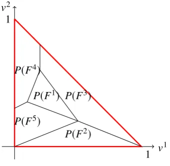
Figure 7. Projection of a three dimensional lower imageDonto thev1-v2coordinate plane.
Figure 7 shows the projection of a three dimensional lower image D onto thev1 and v2 coordinate plane. The cellsP(F1) to P(F5) are the projections of facetsF1 toF5 of D, respectively. Notice that the projections of the facets have disjoint interiors, because by definition D consists of points (v1, . . . ,vp−1,vp) such that vp ≤ v
∗
for the point (v1,vp−1,v∗) ∈ DK, theK-maximal subset ofD.
Definition 6 K-maximal facets Fi and Fj of D are called neighbouring facets if
dim(Fi∩Fj)= p−2.
Figure 7 shows that the neighbouring facets of facetF2areF3 andF5. NeitherF1nor
F4are neighbouring facets ofF2.
Proposition 5 Ifyiandyjare neighbouring vertices ofP, then facetsFi=H∗(yi) ∩ D
andFj =H∗(yj) ∩ Dare neighbouring facets ofD.
Proof. Sinceyiandyjare neighbouring vertices ofYthere is an edge[yi−yj]connecting them. The edge[yi−yj]has dimension one and according to Theorem 3dim([yi−yj])+
dim(Ψ−1([yi − yj])) = p −
1 we have that dim(Ψ−1([yi − yj])) = p −2. Moreover, Ψ−1(yi) = H∗(yi) ∩ D = Fi and Ψ−1(yj) = H∗(yj) ∩ D = Fj due to our notational convention. Hencedim(Fi∩Fj)= p−2andFiandFjare neighbouring facets. Definition 7 Let F be a K-maximal facet of D. If all neighbouring facets of F are K-maximal facets, thenF is called a complete facet, otherwise it is called an incomplete facet. The set of all complete facets ofDis denoted byFc, the set of all incomplete facets ofDis denoted byFic.
In Figure 3 there are two incomplete facets, namely, the facet attached to the origin and the facet attached to the point(1,0)T. The other two facets are complete. In Figure 7 the projections of the incomplete facets areP(F2),P(F3),P(F4)andP(F5). The only complete facet is F1, hence P(F1) is surrounded by the projections of the incomplete facets.
Theorem 7 There exists a one-to-one correspondence between incomplete facets ofD
and incomplete vertices ofP.
Theorem 8 Ify∗is an optimal solution of (8)at an incomplete vertex, then (H∗(y∗) ∩ D)
is aK-maximal incomplete facet ofD.
Proof. Theorem 8 follows directly from Theorem 5 and Theorem 7. Theorem 8 says that a facet ofD corresponding to an optimal extreme point solution to (8) is an incomplete facet. In other words, we do not neeed to investigate complete facets to find an optimal solution because in the primal space the vertex corresponding to this facet has only non-dominated neighbours, i.e., this vertex is a complete vertex, which cannot be an optimal solution of (8). On the other hand, an incomplete facet of Dis the counterpart of an incomplete vertex ofY. Hence an optimal solution to (8) can be obtained by investigating the incomplete facets ofD. In order to obtain the set of incomplete facets ofD, let us define
WD:= p−1
Ø
i=1
v ∈Rp :vi =0,05 vj 5 1,j=1. . .(p−1),j,i
∪
(
v ∈Rp: p−1
Õ
i=1
vi =1,05 vi 51,i=1. . .(p−1)
)
.
In Fig. 7, the highlighted triangle is the projection of WD onto the v1-v2 coordinate plane. The incomplete facets intersect withWD because their neighbouring facets are not all K-maximal facets. On the other hand, a complete facet “surrounded” byK-maximal facets does not intersect withWD. Hence, it is sufficient to consider the facets that intersect withWD. The dual algorithm proposed below is designed to solve (8) in the dual objective space through finding facets that intersect withWD.
Theorem 7 shows that there is a one-to-one correspondence between incomplete vertices ofY and incomplete facets of D. But through intersections withWD incomplete facets ofDare easier to characterise than incomplete facets ofYand can therefore be handled algorithmically.
Algorithm 4Dual algorithm for solving (8). Input: A,b,C, µ
Output: y∗,an optimal solution to (8) Choose some ˆd∈intD.
Compute an optimal solutionx0of (P1(dˆ)), sety ∗
:=C x0,M∗:= µTy∗. SetS0:=
v ∈Rp :λ(v)= 0, p−1
Í
k=1
(yk∗−y∗p)vk−vp = −y∗p
andi:=1. whileWD∩VSk−11 Ddo
Choosevi ∈WD∩VSi−1such thatvi<D.
Compute an optimal solution xiof(P1(vi)), set yi:=C xi. if M∗< µTyithen
Sety∗:= yiandM∗:= µTyi. end if
SetSi :=Si−1∩
v ∈R: p−1
Í
k=1
(yik−yip)vi−vp = −yip
.UpdateVSi.
Seti:=i+1. end while
K-maximal facets need to be generated.
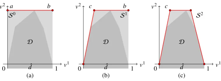
S0
D
0 1 v
1 v2
(a)
a b
ˆ
d
S1
D
0 1 v
1 v2
(b)
b c
ˆ
d
S2
D
0 1 v
1 v2
(c)
c
ˆ
[image:21.595.101.481.135.275.2]d
Figure 8. Iterations of Algorithm 4 in Example 6.
In this example,WD ={v ∈R2:v1 =0} ∪ {v ∈R2:v1=1}. In Figure 8 (a),a,b∈WD. In Figure 8 (b), vertexais used to generate a supporting hyperplane ofD. This hyperplane corresponds to extreme point(0,4)T in the primal space. A new vertex cis found. Since
c <WD, in Figure 8 (c) vertexbis employed to generate another supporting hyperplane
of D corresponding to extreme point(5,0)T in the primal space. At this stage, there is no infeasible vertex belonging toWDand the algorithm terminates with optimal solution (5,0)T.
6.2. The dual algorithm for solving(10)
In Section 6.1, we investigated the properties of (8) in the dual objective space and proposed a dual algorithm to solve (8). The dual Algorithm 4 for (8) determines incomplete K -maximal facets ofD. But since the underlying dual MOP (16) of (10) has a non-polyhedral lower imageD it may have no facets (see Figure 4 for example). However, since the dual variant of Benson’s outer approximation algorithm for solving CMOPs performs an outer approximation toDwe can combine this approximation ofDwith a similar procedure as in Algorithm 4 to solve (10).
Algorithm 5Dual algorithm for solving (10). Input: f,g, µ,
Output: y∗,an optimal solution to (10) and approximate solution to (9). 1: Choose some ˆd ∈intD.
2: Compute an optimal solution x0of (P1(dˆ)), sety ∗
:= f(x0),M∗:= µTy∗. 3: SetS0 :=
v ∈Rp
:λ(v) =0, p−1
Í
k=1
(y∗k−y∗p)vk −vp =−y∗p
andi=1. 4: whileWD∩VSi−1 1DK do
5: Choosesi ∈WD∩VSi−1.
6: Compute an optimal solution xi of(P1(si)) and an optimal value zi to (P1(si)); yi:= f(xi);Mi := µTyi.
7: if M∗< Mithen
8: y∗:= yiandM∗:= Mi. 9: end if
10: ifsip−zi > then 11: SetSi :=Si−1∩
v ∈R: p−1
Í
k=1
(yik−yip)vi−vp = −yip
.UpdateVSi.
12: else
13: VK:=VK∪si. 14: end if
15: Seti:=i+1. 16: end while
Example7 Figure 9 below illustrates the dual algorithm in Example 5.
S0
D
v1 v2
0
a b
(a) ˆ
d
S1
D
v1 v2
0
c b
(b) ˆ
d
S2
D
v1 v2
0
c d
(c) ˆ
[image:22.595.142.437.382.646.2]d
Figure 9. Iterations of Algorithm 5 in Example 7.
to generate another supporting hyperplane to D at (1,0)T resulting in vertex d. Since
c,d < WD, there is no infeasible vertex belonging toWD and the algorithm terminates with the approximate solution y∗ = (3,0)T with value µTy∗ = 15. This is the optimal solution in this example.
7. Computational Results
7.1. The linear case
In this section, we use randomly generated instances to compare some of the algorithms for solving (8). The method proposed by [7] is used to generate instances the coeffi-cients of which are uniformly distributed between -10 and 10. All of the algorithms were implemented in Matlab R2013b using CPLEX 12.5 as linear programming solver. The ex-periments were run on a computer with an Intel i7 processor (3.40GHz and 16GB RAM). We solved three instances of the same size for MOLPs with pobjectives, mconstraints andnvariables. Note thatm= nfor all instances. Table 3 below shows the average CPU times (in seconds). We tested six algorithms, namely
• the brute force algorithm (Algorithm 1), labelled A1
• the bi-objective branch and bound algorithm of Section 4.1, labelled A2 • the conical branch and bound algorithm of Section 4.2, labelled A3 • Benson’s branch and bound algorithm (Section 4.3), labelled A4 • the primal algorithm (Algorithm 2), labelled A5
[image:23.595.108.467.391.667.2]• the dual algorithm (Algorithm 4), labelled A6
Table 3. CPU times of six different algorithms in the linear case.
p m=n A1 A2 A3 A4 A5 A6
5 0.0427 0.0066 0.0128 0.0343 0.0065 0.0147 10 0.0065 0.0016 0.0035 0.0063 0.0068 0.0067 2 50 0.0072 0.0038 0.0282 0.0732 0.0038 0.0084 100 0.0239 0.0069 0.0541 0.1418 0.0197 0.0163 500 0.3226 0.1634 2.5935 12.5185 0.2464 0.2789
5 0.0678 - 0.0074 0.0209 0.0161 0.0269
10 0.0294 - 0.0052 0.0077 0.0114 0.0178
3 50 0.0847 - 0.1005 0.2327 0.0402 0.0386
100 0.1385 - 0.302 0.9642 0.0985 0.0596
500 3.4191 - 3.9931 17.0181 1.4985 0.4342
5 0.1373 - 0.0084 0.0232 0.0637 0.0414
10 0.1951 - 0.1638 0.3575 0.2061 0.0445
4 50 0.5496 - 0.2004 0.066 0.5685 0.1103
100 2.0857 - 3.6578 4.2433 0.7587 0.4348
500 35.8634 - 66.1054 141.241 21.0746 9.1878
5 5.1236 - 0.0934 0.024 0.8902 0.0618
10 2.6293 - 0.0277 0.0099 2.7356 0.1623
5 50 10.9649 - 7.1391 3.249 3.5458 0.8399
100 25.9835 - 50.4573 10.6344 6.4632 2.9714 500 204.7300 - 354.8034 578.1003 89.6327 53.5104
between less than 1 minute and about 10 minutes with p= 5objectives for the different algorithms. We observe that forp=2, the bi-objective branch and bound algorithm turns out to be the fastest algorithm, but it cannot be generalised to problems with more than two objectives. The dimension factor maybe plays a less important role when pis small. Other factors such as the number of variables and constraints may have more influential impact on CPU times. As p increases, the merit of the primal and the dual algorithms is revealed. Specifically, when solving problems with 5 objectives and 500 variables and constraints, the primal and the dual algorithms take much less time (one sixth, respectively one tenth) than Benson’s branch and bound algorithm. The brute force algorithm (A1) performs better than the branch and bound algorithms (A3 and A4) because A1 only solves one LP in each iteration whereas A3 and A4 solve multiple LPs. Solving LPs is the most time-consuming step in the algorithms. Table 3 also shows the dual algorithm performs better than the primal algorithm in solving instances of large scale. In Figure 7.1, we plot the log-transformed CPU times of solving the instances with 500 variables and constraints for the five different applicable algorithms. It shows that, as expected, the time required to achieve optimality exponentially increases with the number of objectives, even for our primal and dual algorithm, making the speed-up obtained by our algorithms even more important.
−1 −0.5 0 0.5 1 1.5 2 2.5 3
2 3 4 5
Log
ar
ithm
of
CPU
time
Number of objectivesp Brute force
+
+
+
+ +
Conical branch and bound
× ×
×
× ×
Benson’s branch and bound
∗ ∗
∗
∗
∗ Primal algorithm
Dual algorithm
[image:24.595.112.458.302.510.2]
Figure 10. Log-transformed CPU times for instances with 500 variables and constraints.
7.2. The convex case
In this section, we use randomly generated instances to compare some of the algorithms discussed in Section 4 and the primal and the dual algorithms for (10). The method proposed by [7] is used to generate convex polyhedra as feasible sets of the underlying CMOP. Quadratic functions are generated as the objective functions, which are in the form
• the brute force algorithm, labelled A1
• the extended bi-objective branch and bound algorithm in Section 4.1, labelled A2 • the conical branch and bound algorithm of Section 4.2, labelled A3
[image:25.595.105.471.141.263.2]• the primal algorithm (Algorithm 3), labelled A4 • the dual algorithm (Algorithm 5), labelled A5
Table 4. CPU times of five different algorithms in the convex case.
p m=n A1 A2 A3 A4 A5
5 2.3037 0.0397 0.2541 0.0821 0.1123
10 4.8086 0.0549 0.4510 0.0869 0.1303
2 50 16.1997 0.4027 1.0291 0.6939 0.4150
100 28.0444 1.8492 2.8614 2.2391 2.0439
5 453.2516 - 246.2019 203.5841 160.5440
10 3821.214 - 2921.345 2061.1652 1631.1805 3 50 17982.2314 - 14669.2419 10621.4219 7243.1480 100 31987.2540 - 24613.2754 18213.4621 13717.6684
Obviously, the CPU time increases rapidly as the size of the instances grows. The largest size of instances we tested is 3 objectives and 100 variables and constraints due to the substantial amount of time required to solve the instances to the chosen accuracy. We notice that the number of objective functions is a crucial factor. All of the instances with p= 2 objectives can be solved within 30 seconds. The most efficient algorithm is the extended bi-objective branch and bound algorithm (A2) proposed by [21], which solves the largest instances with 100 variables and constraints within 2 seconds. Unfortunately it is specific to the bi-objective case. The difference in time between A3, A4 and A5 is not significant. We notice that adding one more dimension to the objective space (i.e., adding one more objective function) leads to substantial increase in computational effort. For instances with 3 objectives, the required CPU time increases substantially so that even instances with 5 variables and constraints take a few minutes to solve. Furthermore, the largest instances with 100 variables and constraints, take a few hours. The dual algorithm solves the largest instances in half of the time used by the conical branch and bound algorithm (A3). We also notice that the dual algorithm is faster than the primal one in most of the cases. Throughout the test, the slowest algorithm is the brute force algorithm (A1). This is due to the fact that this algorithm enumerates a large number of vertices which are redundant. This also proves the advantage of the techniques employed in our new algorithms. Additionally, in the implementation of the algorithms, we notice that time required to solve instances is sensitive to the approximation accuracy (reflected by as stated in the algorithms). In this test the level of accuracy is 10−4. It is expected that a lower level of accuracy results in faster solution time.
8. Conclusion
set to reduce the need for complete enumeration of all non-dominated extreme points. We have compared our algorithms to several algorithms from the literature, and the complete enumeration approach, and obtained speed-ups of up to 10 times on instances with up to 5 objectives and 500 variables and constraints.
We also extended the primal and the dual algorithms to optimise a linear function over the non-dominated set of a convex multi-objective optimisation problem. We employed the techniques of the linear primal and dual methods to facilitate the non-linear ones. Comparing with other algorithms from the literature, our primal and dual algorithms are the fastest. In the future we plan to address more challenging versions of this problem, e.g. when the function to be optimised is nonlinear and when the underlying MOP is nonconvex, where we are particularly interested in the discrete case.
Acknowledgments and Data Statement
We express our gratitude to two anonymous referees, whose careful reading and comments helped us improve the paper. This research was supported by grant FA8655-13-1-3053 of the US Airforce Office for Scientific Research. More information on the data can be found at doihttps://dx.doi.org/10.17635/lancaster/researchdata/224.
References
[1] Benson, H. (1995). A geometrical analysis of the efficient outcome set in multiple objective convex programs with linear criterion functions.Journal of Global Optimization, 6(3):231–251. [2] Benson, H. (1998). An outer approximation algorithm for generating all efficient extreme points in the outcome set of a multiple objective linear programming problem. Journal of
Global Optimization, 13:1–24.
[3] Benson, H. (2011). An outcome space algorithm for optimization over the weakly efficient set of a multiple objective nonlinear programming problem. Journal of Global Optimization, 52(3):553–574.
[4] Benson, H. and Lee, D. (1996). Outcome-based algorithm for optimizing over the efficient set of a bicriteria linear programming problem.Journal of Optimization Theory and Applications, 88(1):77–105.
[5] Benson, H. P. (1984). Optimization over the efficient set. Journal of Mathematical Analysis
and Applications, 98(2):562–580.
[6] Benson, H. P. (1991). An all-linear programming relaxation algorithm for optimizing over the efficient set.Journal of Global Optimization, 1(1):83–104.
[7] Charnes, A., Raike, W. M., Stutz, J. D., and Walters, A. S. (1974). On generation of test problems for linear programming codes.Communications of the ACM, 17(10):583–586. [8] Dauer, J. (1993). On degeneracy and collapsing in the construction of the set of objective values
in a multiple objective linear program.Annals of Operations Research, 46-47(2):279–292. [9] Dauer, J. P. (1987). Analysis of the objective space in multiple objective linear programming.
Journal of Mathematical Analysis and Applications, 126(2):579–593. [10] Ehrgott, M. (2005). Multicriteria Optimization (2. ed.). Springer, Berlin.
[11] Ehrgott, M., Güler, Ç., Hamacher, H. W., and Shao, L. (2009). Mathematical optimization in intensity modulated radiation therapy.Annals of Operations Research, 175(1):309–365. [12] Ehrgott, M., Löhne, A., and Shao, L. (2011). A dual variant of benson,s uter
approxima-tion algorithm for multiple objective linear programming. Journal of Global Optimization, 52(4):757–778.
[13] Ehrgott, M., Naujoks, B., Stewart, T. J., and Wallenius, J. (2010). Multiple Criteria Decision
Making for Sustainable Energy and Transportation Systems, volume 634 of Lecture Notes in Economics and Mathematical Systems. Springer, Berlin.
Decision Analysis: State of the Art Surveys, volume 78 ofInternational Series in Operations
Research and Management Science, pages 667–708. Springer New York.
[15] Fruhwirth, M. and Mekelburg, K. (1994). On the efficient point set of tricriteria linear programs.European Journal of Operational Research, 72:192–199.
[16] Fülöp, J. (1993). On the equivalency between a linear bilevel programming problem and linear optimization over the efficient set. Technical report, Hungarian Academy of Sciences. [17] Fülöp, J. and Muu, L. D. (2000). Branch-and-bound variant of an outcome-based algorithm
for optimizing over the efficient set of a bicriteria linear programming problem. Journal of
Optimization Theory and Applications, 105(1):37–54.
[18] Hamel, A., Löhne, A., and Rudloff, B. (2014). Benson type algorithms for linear vector optimization and applications.Journal of Global Optimization, 59(4):811–836.
[19] Heyde, F. and Löhne, A. (2008). Geometric duality in multiple objective linear programming.
SIAM Journal on Optimization, 19(2):836–845.
[20] Horst, R. and Tuy, H. (1993). Global Optimization: Deterministic Approaches. Springer, Berlin.
[21] Kim, N. T. B. and Thang, T. N. (2013). Optimization over the efficient set of a bicriteria convex programming problem.Pacific Journal of Optimization, 9:103–115.
[22] Löhne, A., Rudloff, B., and Ulus, F. (2014). Primal and dual approximation algorithms for convex vector optimization problems.Journal of Global Optimization, 60(4):713–736. [23] Markowitz, H. (1952). Portfolio selection*. The Journal of Finance, 7(1):77–91.
[24] Thoai, N. V. (2000). Conical algorithm in global optimization for optimizing over efficient sets.Journal of Global Optimization, 18(4):321–336.
[25] Yamamoto, Y. (2002). Optimization over the efficient set: overview. Journal of Global
Optimization, 22(1-4):285–317.