warwick.ac.uk/lib-publications
Original citation:
Gulpinar, Nalan and Çanakoḡlub, Ethem . (2016) Robust portfolio selection problem under temperature uncertainty. European Journal of Operational Research.
Permanent WRAP URL:
http://wrap.warwick.ac.uk/79816
Copyright and reuse:
The Warwick Research Archive Portal (WRAP) makes this work by researchers of the University of Warwick available open access under the following conditions. Copyright © and all moral rights to the version of the paper presented here belong to the individual author(s) and/or other copyright owners. To the extent reasonable and practicable the material made available in WRAP has been checked for eligibility before being made available.
Copies of full items can be used for personal research or study, educational, or not-for-profit purposes without prior permission or charge. Provided that the authors, title and full bibliographic details are credited, a hyperlink and/or URL is given for the original metadata page and the content is not changed in any way.
Publisher’s statement:
© 2016, Elsevier. Licensed under the Creative Commons Attribution-Non
Commercial-NoDerivatives 4.0 International http://creativecommons.org/licenses/by-nc-nd/4.0/
A note on versions:
The version presented here may differ from the published version or, version of record, if you wish to cite this item you are advised to consult the publisher’s version. Please see the ‘permanent WRAP URL’ above for details on accessing the published version and note that access may require a subscription.
Accepted Manuscript
Robust Portfolio Selection Problem under Temperature Uncertainty
Nal ˆan G ¨ulpınar, Ethem C¸ anako ¯glu
PII: S0377-2217(16)30383-6 DOI: 10.1016/j.ejor.2016.05.046
Reference: EOR 13732
To appear in: European Journal of Operational Research
Received date: 5 May 2015 Revised date: 29 March 2016 Accepted date: 26 May 2016
Please cite this article as: Nal ˆan G ¨ulpınar, Ethem C¸ anako ¯glu, Robust Portfolio Selection Prob-lem under Temperature Uncertainty, European Journal of Operational Research (2016), doi:
10.1016/j.ejor.2016.05.046
ACCEPTED MANUSCRIPT
Highlights
• A portfolio selection problem under temperature uncertainty is studied.
• CVaR portfolio optimization is considered for scenario-based uncertainty set.
• Robust counterparts of the problem are derived using advanced uncertainty sets.
• Risk references are incorporated in the suggested robust framework.
ACCEPTED MANUSCRIPT
Robust Portfolio Selection Problem under Temperature Uncertainty
Nalˆan G¨ulpınara, Ethem C¸ anako¯glub
aThe University of Warwick, Warwick Business School, Coventry, CV4 7AL, UK. bBah¸ce¸sehir University, Industrial Engineering, Istanbul, Turkey.
Abstract
In this paper, we consider a portfolio selection problem under temperature uncertainty. Weather deriva-tives based on different temperature indices are used to protect against undesirable temperature events. We introduce stochastic and robust portfolio optimization models using weather derivatives. The investors’ different risk preferences are incorporated into the portfolio allocation problem. The robust investment decisions are derived in view of discrete and continuous sets that the underlying uncertain data in temper-ature model belong. We illustrate main fetemper-atures of the robust approach and performance of the portfolio optimization models using real market data. In particular, we analyze impact of various model parameters on different robust investment decisions.
Keywords: Robust investment decisions, temperature uncertainty, asset allocation, weather derivatives
1. Introduction
Weather plays a significant role in determining revenue of some industries and market players. National Science Foundation estimated the annual economic impact of weather risk to the US economy as $485 billion in 2011. Various business sectors such as agriculture, retail, tourism and energy are directly affected by exceptional weather conditions (Svec and Stevenson (2007)). For instance, a warm winter may cause excess supplies of oil or natural gas for the utility and energy companies or may incur significant losses in earnings of a winter resort. Similarly, an exceptionally cold summer can affect tourism sector in various aspects. Even big construction companies, especially in Northern Europe, with tight deadlines and costly penalty clauses, consider derivatives to hedge the risk of delays due to weather conditions (The Economist Magazine (2012)).
Weather derivatives were first introduced by Enron in 1997 as financial instruments to minimize effects of climatic events in the US energy industry. Since then, the unregulated market for temperature derivatives has been constantly growing. The standardized contracts are also available in Chicago Mercantile Exchange (CME) for the major cities in the USA, Europe, Australia and Japan. The most common weather derivatives are written on temperature indices that form about 80% of weather contracts to manage weather related risk (Cao and Wei (2004)). There are also weather contracts written on other weather events such as levels of rain, snow, wind, frost and hurricanes.
The pricing problem for weather derivatives has been widely studied in the literature; for instance see Jewson and Brix (2005), Benth and Saltyte-Benth (2007 and 2011), Dorfleitner and Wimmer (2010),
∗Corresponding author
ACCEPTED MANUSCRIPT
Schiller et al. (2012), and Hardle et al. (2012). The underlying indices or degree days are modeled under an assumption of various stochastic processes. Garman et al. (2000) and Svec and Stevenson (2007) modeled the underlying indices of weather derivatives using both time series and stochastic approaches. Brody et al. (2002) characterized temperature dynamics by a fractional Ornstein-Uhlenbeck process to price contingent claims based on heating and cooling-degree-days. Hamisultane et al. (2010) studied utility based pricing of weather derivatives. Recently, Elias et al. (2014) compared regime-switching temperature modelling approaches for applications in weather derivatives. The reader is referred to Saltyte-Benth and Benth (2012) for a critical review on temperature modelling.
mean-ACCEPTED MANUSCRIPT
variance portfolio allocation framework to handle uncertainty arising due to misspecification and estimation errors for (mainly means and covariance matrices of) random asset returns: for instance see Goldfarb and Iyengar (2003), Ceria and Stubbs (2006), and Kawas and Thiele (2009). Moon and Yao (2011) showed that effective portfolio allocation strategies can be obtained by careful selection of the uncertainty sets over which the worst-case is considered. Soyster and Murphy (2013) introduced a framework for duality and modelling in robust linear programs and applied to the classic Markowitz portfolio selection problem. Oguzsoy and Guven (2007) studied robust portfolio planning problem in the presence of market anomalies. In addition, there exists several successful applications of the robust optimization approach within the multi-period portfolio allocation framework; for instance, see Ben-Tal et al. (2002) and Bertsimas and Pachamanova (2008).
Robust optimization considers the worst-case decision criteria, unlike the expected value criteria is used as a standard approach for decision making problems under uncertainty. It possesses modelling and compu-tational advantages over the stochastic programming, Ben-Tal and El Ghaoui (2009). The data uncertainty is taken into account during modeling stage of the problem without an assumption on specific distribution of the underlying random variables. The uncertain parameters take their worst-case values within a set (so-called an uncertainty set). An uncertainty set consists of general restrictions (representing different forms of rules or factors) on the realizations of the uncertainties of the underlying stochastic program. The robust counterpart of the stochastic program is derived in view of the pre-specified uncertainty set. This is a deterministic model that does not involve an uncertain parameter, Bertsimas et al., (2004). Most impor-tantly, the robust model becomes computationally tractable. The main drawback of the robust optimization methodology is that specific choice of uncertainty sets and budget of robustness may lead to a conservative strategy (Gulpinar and Rustem (2007)). The recent studies showed that data driven robust approaches to design uncertainty sets utilizing data can overcome this issue and avoid overly conservative strategies; see for instance, Bertsimas et al. (2013).
In this paper, we are concerned with a portfolio management problem under temperature uncertainty using weather derivatives. A robust optimization approach to portfolio allocation of weather derivatives is introduced to investigate impact of temperature noise on the investment strategies. We are particularly interested in the effect of robust investment strategies for insurance purposes, that is, whether robust op-timization strategies perform better than traditional strategies in extreme scenarios. We present robust formulations of the portfolio allocation problem under different uncertainty sets to incorporate risk prefer-ences of the investor. We therefore consider discrete (scenario-based) as well as continuous (symmetric and asymmetric) uncertainty sets for modelling temperature uncertainty. Specifically, we introduce Conditional Value-at-Risk (CVaR) constraints using scenario-based uncertainty set in the context of portfolio selection problem under weather uncertainty. The symmetric and asymmetric uncertainty sets in view of certain conditions determine a risk measure on the uncertainty arising in the underlying problem. For further infor-mation on the use of risk measures in financial applications, the reader is referred to Rockafellar and Uryasev (2000) and Natarajan et al. (2008). The numerical experiments are conducted to analyze performance of different investment strategies determined in view of different risk preferences and to investigate impact of various model parameters on the performance of robust investment decisions using real data.
ACCEPTED MANUSCRIPT
temperature uncertainty is introduced in Section 4. In Section 5, we derive robust portfolio formulations using different uncertainty sets. Section 6 summarizes design of numerical experiments, implementation issues and data analysis . We present an empirical analysis of robust weather investment strategies using real market data and computational results in Section 7. Section 8 concludes the paper with a short summary of findings and future research directions.
2. Weather Derivatives
Weather derivatives are traded as financial instruments between two parties. The seller agrees to bear risk for a premium and makes profit if nothing happens. However, if the weather turns out to be bad, then the buyer claims the agreed amount. Broadly speaking, futures (forwards) and options are main types of weather derivatives that are written on temperature indices. The reader is referred to Jewson (2002) for further discussion on different weather derivatives. Besides the underlying variable of temperature indices, a weather contract must specify such basic elements as the accumulation period, the index location (which records temperatures used to construct the underlying variable), and the tick-size (i.e., fixed lump-sum to be exchanged between parties for each level of degree days). The weather indices are defined through temperature realised at any day for a specific location. The products associated with regions located in the same geographical region are highly correlated. In this sense, a portfolio allocation problem using weather derivatives displays different characteristics from other commodity types such as oil and corn.
We consider weather futures and options based on temperature indices associated withmlocations that are indexed by i, j = 1,· · ·, m. Let T denote an investment horizon and t represent future discrete time periods,t= 1,2,· · ·, T. We assume thatt= 0 refers to today. Let ˜Hit represent the temperature measured
for location i= 1,· · ·, mat timet= 1,· · ·, T. The temperature at a specific day is basically average of the highest and lowest temperatures observed during the day.
A degree day is defined as the difference between a reference temperature and the daily observed tem-perature. The temperature indices are described by heating-degree-days (HDD) and cooling-degree-days (CDD) and cumulative average temperature (CAT). In general terms, the HDD (CDD) indices are used to measure coldness (hotness) of the temperature during a period of November-March (April-November). Let ri be the reference temperature associated with locationi. In general, it is fixed as 18 degrees Celsius
or 65 degrees Fahrenheit. The HDD and CDD indices, respectively, at time t for location i are defined as temperatures below and over the reference temperature ri, and are formulated as
HDD(i, t) = max(ri−H˜it,0), and CDD(i, t) = max( ˜Hit−ri,0).
The total heating and cooling-degree-days for HDD and CDD indices associated with location i over time period T are mathematically formulated as
fi= T
X
t=1
HDD(i, t), and gi= T
X
t=1
CDD(i, t).
In addition, total daily average temperatures with respect to CAT index at locationiduring the measurement
period T is calculated asdi= T
X
t=1
CAT(i, t) =
T
X
t=1 ˜
ACCEPTED MANUSCRIPT
Let ¯fi, ¯gi and ¯di denote the level of degree days agreed between the parties for HDD, CDD and CAT
indices at location i, respectively. A weather futures contract obligates the buyer to purchase the value of underlying temperature index at a future date based on the accumulated heating or cooling-degree-days. The parties exchange the value of the contract at the end of investment horizon. The payoff received from the weather futures contracts on HDD, CDD and CAT temperature indices for location i, respectively, is expressed as
FHDD(i) =phi(fi−f¯i), FCDD(i) =pci(gi−g¯i), and FCAT(i) =pcti (di−d¯i)
where ph
i, pci and pcti are tick-sizes attached to HDD, CDD, and CAT indices, respectively, for location i.
In the CME market, various weather options written on temperature futures are also traded. A call (put) option provides its owner the right to buy (sell) the underlying asset for a fixed strike price at an agreed exercise time. The underlying asset is a temperature future written on temperature (HDD, CDD or CAT) indices for a specified measurement period.
Let Kh
i andKic denote strike prices of HDD and CDD indices, respectively. The value of a weather call
option with underlying futures temperatures written on heating and cooling-degree-days, respectively, for location i is determined as
CHDD(i) =phi max
fi−Kih,0
, and CCDD(i) =pcimax (gi−Kic,0).
Similiarly, the value of a weather put option on futures temperatures written on heating and cooling-degree-days for location ican be computed as follows:
PHDD(i) =phi max
Kih−fi,0
, and PCDD(i) =pcimax (Kic−gi,0).
Therefore, it is desirable for an investor to exercise the call (put) option when the strike price on the option contract is lower (higher) than the market value of the underlying temperature indices.
Next, we first describe the temperature model based on autoregressive process, and then introduce a stochastic portfolio selection model under temperature uncertainty using weather future derivatives. Weather options can be also included in a similar manner.
3. Modelling Temperature Uncertainty
ACCEPTED MANUSCRIPT
We use notation tilde to represent randomness; for example, (˜∗) denotes a random variable (∗). Let’s assume that the trader knows the temperature values today (t = 0), but temperature ˜Hit for location in
future time periodstfort >0 are unknown (uncertain). The temperature dynamics for locationiat time t
can be modeled as
˜
Hit=µit+δit
where µit and δit represent the mean and the residual process at time t for location i, respectively. As
suggested by Saltyte-Benth and Benth (2012), the auto-regressive process AR of order 3 is the best fit for modelling the cyclic component of temperature data. Let lki for k = 1,2,3 at location i denote the
parameters ofAR(3). The mean process is defined in terms of the seasonal and mean reverting components as follows;
µit=sit+
3 X
k=1
lki
˜
Hit−k−sit−k
. (1)
The seasonal mean function is deterministic and contains a trend and the seasonality of temperature data. It can be formulated as follows;
sit=a0i+a1it+a2icos
2π(t−a3i)
365
.
The first component (a0i) in the seasonality function of temperature represents the long-term average
tem-perature for location i whereas the trend line (a1it) is used to ensure stationarity in temperature data. A
trend could be expressed as an increasing temperature due to for instance, global warming (Saltyte-Benth and Benth (2012)). The trigonometric function in the last component refers the seasonal variation in tem-perature and changes between the coldest and the warmest periods of the year. The size of variation is equal to two times a2i while a3i denotes the phase variable for the trigonometric function which corresponds to
the hottest day in the year.
As shown by the temperature data analysis in Section 6, and also reported in the literature (for instance, see Alaton et al. (2002)), the temperature data suggests that the variability in the residual process δit is
not an independent identically distributed random variable. On the other hand, it depends on the season and also captures correlation of temperatures between all locations (Barth et al. (2011)). Let ρit be the
seasonal variation andΣ represent am×mmatrix with elements of σij whereΣ0Σ is the covariance of the
normalized residuals.
Therefore, we can model the residual process as
δit=ρit m
X
j=1
σijε˜jt. (2)
where ˜εjt represents independent random noise. The temperature data analysis in Section 6 proves that the
noise term follows a distribution with zero mean and 1 standard deviation.
We model the seasonal volatility using Fourier transform function with a single component defined as
ρit=b0i+b2icos
2π(t−b3i)
365
ACCEPTED MANUSCRIPT
Note that time independent random process exhibit spatial dependence and is used to model the correlation of temperature changes in different locations. This component is modeled as the summation of independent
random processes as
m
X
j=1
σijε˜jt. Therefore, temperature of locationi at time tcan be rewritten as
˜
Hit=sit+
3 X k=1 lki ˜
Hi,t−k−si,t−k
+ρit
m
X
j=1
σijε˜jt.
Let’s assume that the temperature values for 3 days prior to current day, Hi(−2), Hi(−1), Hi(0), and seasonal components for that period, si(−2), si(−1), si(0), for locationi are known. Using the backward induction and some algebra, one can obtain the temperature at time tfor location i as a function of the temperatures at the beginning of decision period (namely,Hi(−2), Hi(−1), and Hi(0)) and can be written as follows:
˜
Hit=sit+
3 X
k=1
Akit Hi(1−k)−si(1−k)+
t
X
k=1
A1i(t−k)ρit m
X
j=1
σijε˜jk, (3)
where A1it = X
∀a+2b+3c=t
la1ilb2ilc3i, A2it = A1i(t+1)−A1itl1i, and A3it = A1i(t+2)−A1i(t)l2i−A2i(t+1)l1i. The total
heating-degree-days for HDD and CDD temperature indices over a planning horizonT are computed as
fi = T
X
t=1 max
ri−sit−
3 X
k=1
Akit Hi(1−k)−si(1−k)−
t
X
k=1
A1i(t−k)ρit m
X
j=1
σijε˜jk, 0
, and (4)
gi = T
X
t=1 max
sit+
3 X
k=1
Akit Hi(1−k)−si(1−k)+
t
X
k=1
A1i(t−k)ρit m
X
j=1
σijε˜jk−ri, 0
. (5)
4. Stochastic Portfolio Allocation under Temperature Uncertainty
We assume that an investor (a firm, a hedge fund or an insurance company) is concerned with weather risk and wishes to construct a portfolio using weather derivatives traded in the CME market. Moreover, the investor considers two types of futures contracts in the market where temperature is the underlying index for weather futures (written on HDD and CDD temperature indices over a given measurement period). Let xhi and xci be decision variables representing weights of the futures contracts written on heating and cooling-degree indices for location i, respectively. The capital is normalized to unity so that we have
m
X
i=1
xhi +xci = 1 (6)
where non-negativity constraints on asset weights, xhi, xci ≥0 fori = 1,· · ·, maim to avoid the short-sale. The expected terminal wealth obtained from an investment of weather futures written on HDD and CDD temperature indices for locationi is computed as
Ehxhiphi fi−f¯i+xcipci(gi−¯gi)
ACCEPTED MANUSCRIPT
Recall that phi andpci define the tick sizes for HDD and CDD contracts, respectively. The investor’s goal is to maximize the total expected wealth that is achieved by the investment on HDD and CDD weather futures associated with locationsi= 1,· · ·, m. Then the stochastic portfolio allocation problem can be formulated as follows;
Pnom: max xh
i,xci
m
X
i=1
Ehxhiphi fi−f¯i+xcipci(gi−g¯i)
i
s.t. fi= T
X
t=1 max
ri−sit−
3 X
k=1
Akit Hi(1−k)−si(1−k)
−
t
X
k=1
A1i(t−k)ρit m
X
j=1
σijε˜jk, 0
,
i= 1,· · ·, m
gi= T
X
t=1 max
sit+
3 X
k=1
Akit Hi(1−k)−si(1−k)+
t
X
k=1
A1i(t−k)ρit m
X
j=1
σijε˜jk−ri, 0
,
i= 1,· · ·, m
m
X
i=1
xhi +xci = 1
xh
i ≥0, xci ≥0, i= 1,· · ·, m.
Notice that fi andgi functions (in the first and second sets of equations) are written explicitly rather than
substituting in the objective function due to convenience since the uncertain parameters arising in these equations will be robustified in the upcoming sections.
The solution of the single-period portfolio selection model with recourse determines an optimal allocation of wealth among temperature derivatives written on heating and cooling indices. The optimal investment decision is made at the beginning of the investment horizon and total wealth received from the investment depends on the path the temperature following between today t = 0 and final time period T like some exotic options. As mentioned earlier, a stochastic programming model assumes that the decision maker is concerned with the average performance of the system. Moreover, it requires a known distribution of the underlying uncertainty. The expected wealth, formulated in terms of contributions of weather futures under consideration, inPnom can be easily computed by estimating expected return of each weather futures under
an assumption of specific noise distribution. Then the stochastic programming model above becomes a simple linear programming problem that supplies the investment strategy to achieve maximum portfolio return. Similarly, we can construct a scenario-based stochastic programming model to maximize the expected wealth with discrete number of future temperature scenarios that are generated by the underlying distribution of random parameters. Both approaches provide risk-neutral strategies. On the other hand, for the risk-seeking investment decisions, the expected risk needs to be specifically modeled and minimized for the optimal portfolio allocation. In this paper, we consider conditional Value-at-Risk (CVaR) metric and analyze the risk factor for CVaR constraints in the context of temperature risk management. The alternative risk preferences of the investor will be imposed through robust approaches in the next section.
Following Rockafellar and Uryasev (2000), the Conditional Value-at-Risk measure for a random variable ˜
v,ρ1−(˜v), is defined as
ρ1−(˜v) = min a
a+1
E(−v˜−a)
ACCEPTED MANUSCRIPT
that can be reformulated by a set of the CVaR constraints in view of N discrete scenarios of ˜vas
Ucvar(v) =
(
µ+ 1
b(1−δ)·Nc
N
X
n=1
βn ≤Cδ, −µ−βn ≤f(˜v), βn≥0, n= 1, . . . , N
)
where b·c denotes the integer part of a real number and Cδ is a predetermined constant and f(˜v) is the
loss function. It is worthwhile to mention that the set of CVaR constraints constructs a scenario-based uncertainty set in the context of robust optimization; for instance see Bertsimas et al. (2013).
The CVaR portfolio optimization model under weather derivatives considers K realisations of random temperature. For each realisation ¯k = 1, . . . , K and futures i = 1,· · ·, m, we can compute γk¯
i, and δ
¯
k i as
follows;
γi¯k =
T
X
t=1 max
ri−sit−
3 X
k=1
Akit Hi(1−k)−si(1−k)−
t
X
k=1
A1i(t−k)ρit m
X
j=1
σijεkjk¯ , 0
, and
δi¯k =
T
X
t=1 max
sit+
3 X
k=1
Akit Hi(1−k)−si(1−k)+
t
X
k=1
A1i(t−k)ρit m
X
j=1
σijεkjk¯ −ri, 0
.
The expected portfolio return over K scenarios must be at least at the target levelWtarget. This condition
is basically formulated as follows:
K X ¯ k=1 1 K m X i=1
xhiphi γi¯k−f¯i
+xcipciδki¯−g¯i
≥Wtarget.
The CVaR portfolio allocation problem with conditional performance constraint on weather derivatives can be formulated as follows:
Pcvar: min Γ
s.t. µ+ 1
b(1−β)·Kc
K
X
¯
k=1
u¯k ≤Γ,
uk¯≥ −
m
X
i=1 h
xhiphi γik¯−f¯i
+xcipciδi¯k−¯gi
i
−µ, k¯= 1, . . . , K
K X ¯ k=1 1 K m X i=1
xhiphi γki¯−f¯i
+xcipciδ¯ki −g¯i
≥Wtarget,
uk¯≥0, xci ≥0, xih ≥0 i= 1,· · ·, m, ¯k= 1, . . . , K.
The CVaR minimization (or maximization) model imposes single objective to find an optimal investment strategy for minimum risk (or maximum wealth) portfolio in view of risk preferences of the investor. The multi-objective formulation produces a minimum risk investment strategy to achieve pre-determined wealth
Wtarget. Notice thatPcvar is a linear programming model whose size (in terms of number of constraints and
variables) depends on the number of assets as well as the number of scenarios generated.
ACCEPTED MANUSCRIPT
probabilistic guarantees on the optimal solution, robust optimization may be a plausible approach since it takes into account investors’ risk preferences and provides a guaranteed performance at the worst-case.
5. Robust Investment Decisions using Weather Contracts
We assume that uncertain parameters ˜εt vary within an uncertainty setUε. The robust counterpart of
the stochastic portfolio management problem optimizes the worst-case wealth over a given uncertainty set for the random variables and can be formulated as
Prob: max xh
i,xci
min ˜
εit∈Uε
m
X
i=1
xhiphi
T
X
t=1
γit+ xcipci T
X
t=1
δit− xhiphif¯i− xcipcig¯i
!
s.t. γit= max
ri−sit−
3 X
k=1
Akit Hi(1−k)−si(1−k)
−
t
X
k=1
A1i(t−k)ρit m
X
j=1
σijε˜jk, 0
, i= 1,· · ·, m,
t= 1,· · ·, T
δit= max
sit+
3 X
k=1
Akit Hi(1−k)−si(1−k)+
t
X
k=1
A1i(t−k)ρit m
X
j=1
σijε˜jk−ri, 0
, i= 1,· · ·, m,
t= 1,· · ·, T
m
X
i=1
xhi +xci = 1, xhi ≥0, xci ≥0, i= 1,· · ·, m.
The max (a,0) function (in the first and second sets of constraints of the minimax problem above) takes either positive value of function a or zero. Therefore, it can be represented by a constraint asy≥ a where
y≥0. Let Γ be a free variable representing the worst-case portfolio wealth in view of ˜εit∈Uε. We can show
that the optimization problem above is equivalent to
max
xh
i,xci,Γ
Γ−
m
X
i=1
xhiphif¯i−xcipci¯gi
s.t. Γ≥
m X i=1 T X t=1
xhiphiγit+xcipci δit,
γit≥ri−sit−
3 X
k=1
Akit Hi(1−k)−si(1−k)
−
t
X
k=1
A1i(t−k)ρit m
X
j=1
σijε˜jk, i= 1,· · ·, m,
t= 1,· · ·, T
δit≥sit+
3 X
k=1
Akit Hi(1−k)−si(1−k)
+
t
X
k=1
A1i(t−k)ρit m
X
j=1
σijε˜jk−ri, i= 1,· · ·, m,
t= 1,· · ·, T
˜
εit∈Uε, γit, δit≥0, i= 1,· · ·, m, t= 1,· · ·, T
m
X
i=1
xhi +xci = 1, xhi ≥0, xci ≥0, i= 1,· · ·, m.
The worst-case outcome of the stochastic data ˜εit within a pre-specified uncertainty set Uε is derived and
ACCEPTED MANUSCRIPT
parameters. The important issue is how to construct an uncertainty set so that random behaviour of the data is well captured, and, at the same time, its robust counterpart should be solved efficiently, in the most computationally tractable way. As Bertsimas et al. (2004) highlighted, an uncertainty set can be determined by statistical estimates and probabilistic guarantees for the solution. The random data that belongs to an uncertainty set is mapped out from the probability distribution of uncertain factors. The support of the random variables can be approximated by using different shapes of the uncertainty sets such as ellipsoidal, box and polyhedral that have been widely used in different applications in the literature. In this paper, we consider symmetric (ellipsoidal) and asymmetric uncertainty sets (introduced by Chen et al. (2007)) to find the corresponding robust counterpart of the asset allocation problem in the context of risk management. The CVaR optimization approach under the scenario-based uncertainty set takes into account the investor’s risk preferences. Recall that the scenario-based uncertainty set, that is already defined (in Section 4) for the CVaR risk optimization model, will be used as a benchmark to compare with the performance of risk-seeking investors’ robust strategies.
It is worthwhile to mention that the size and shape of the uncertainty sets play an important role on performance of the robust strategies. The size of the uncertainty set is often related to guarantees on the probability that the constraint involving uncertain coefficients will not be violated. There is a trade-off between the amount of protection against uncertainty that is desired and optimality - the smaller the probability that the constraint will be violated, the more the modeller gives up in terms of optimality of the robust solution relative to the solution to the original optimization problem.
The shape of the uncertainty set defines a risk measure on the constraints with uncertain coefficients; for instance, see Natarajan et al. (2009). In practice, the shape is selected to reflect the modeler’s knowledge of the probability distributions of the uncertain parameters, while at the same time making the robust counterpart problem efficiently solvable. The symmetric (e.g. ellipsoidal) uncertainty set defines a standard-deviation-like risk measure on the constraint with uncertain parameters. The uncertainty sets with a specific asymmetric shape that incorporates knowledge about the skewed probability distributions of the underlying random asset returns, can improve the performance of investment decisions under Value-at-Risk type risk measures on the portfolio return (Natarajan et al. (2008)). On the other hand, a symmetric uncertainty set with an ellipsoidal shape can be interpreted as variance type risk measures (Fabozzi et al. 2007).
We now focus on robust formulations of the portfolio allocation problem for weather derivatives using symmetric and asymmetric uncertainty sets.
Symmetric Uncertainty Set: In general terms, an ellipsoidal uncertainty set describes a distance requirement - the form of the Euclidean norm - between all elements of the set and the point estimates of the uncertain data. For random variables ˜εt = [˜ε1t,ε˜2t,· · ·,ε˜mt], we can mathematically define ellipsoidal
uncertainty set UE as
UE =
n ˜
εt |
Q−1/2(˜εt−εˆt)
2≤κ o
, (7)
where matrix Q denotes an estimated covariance matrix andεˆt is an expected value of the distribution of
random variables ˜εt. In addition, radiusκmeasures the level of the robustness (sometimes referred to as the
ACCEPTED MANUSCRIPT
of the solution for the underlying problem.
For random variables ˜εt = {ε˜1t,ε˜2t,· · ·,ε˜mt}, at time period t = 1,· · ·, T, we have ˆεt = 0 and Q=I.
In this case, the ellipsoidal set for error terms at time tis simplified asUE ={ε˜it:kε˜tk2≤κ}. Letαit and
βit be Lagrangian multipliers associated with constraints inRnom. In addition, let’s define a vectorBt of
Bt(i) = T
X
k=t
(αik−βik)A1i(t−k)ρitfori= 1,· · ·, mandt= 1,· · ·, T. The robust counterpart of the underlying
stochastic program using the ellipsoidal uncertainty set can be derived as in the following theorem.
Theorem 1. The robust counterpart of the portfolio allocation problem under the symmetric uncertainty set using futures weather contracts with heating and cooling-degree-days can be formulated as
Rsym: max Π− m
X
i=1
xhiphif¯i+xcipci¯gi
s.t.
m
X
i=1
T
X
t=1
(αit−βit) ri−sit−
3 X
k=1
Akit Hi(1−k)−si(1−k)
!
−κ
T
X
t=1
kΣtBtk2 ≥Π
m
X
i=1
xhi +xci = 1
xh
iphi −αit≥0, i= 1,· · ·, m, t= 1,· · ·, T
xc
ipci −βit≥0, i= 1,· · ·, m, t= 1,· · ·, T
xhi ≥0, xci ≥0, i= 1,· · ·, m
αit, βit≥0, i= 1,· · ·, m, t= 1,· · ·, T .
As shown in Appendix B, a formal proof of Theorem 1 derives the robust counterpart of the corre-sponding problem. This process requires to solve (inner) optimization problems that find the worst-case values of the terms involving uncertain coefficients when these uncertain coefficients vary in the uncertainty sets. Notice that in case of the ellipsoidal uncertainty sets with zero means and the unity covariance ma-trices of the uncertain error coefficients, the robust counterparts of the constraints involve the square root terms. Therefore, the robust portfolio allocation model is a second-order-cone programming problem. An explanation of the specific optimization setup used for numerical experiments will be provided in Section 6. The computational experience shows that symmetric uncertainty sets for the uncertain asset returns in the portfolio optimization problem could lead to a highly conservative strategy, especially when the random parameters possess skewed distributions, Ceria and Stubbs (2006). In other words, the asymmetric characteristics of distribution may not be well captured by the symmetric uncertainty set. In order to deal with this issue, Chen et al. (2007) introduced an asymmetric uncertainty set using a factor-based model to represent forward and backward deviations of the random variables in the underlying application. They showed that the asymmetric uncertainty set represents a generic convex uncertainty set (ellipsoidal) when the underlying random variable follows a normal distribution. Next, we will give a brief overview of this approach and present the robust formulation of the portfolio management of weather derivatives using an asymmetric uncertainty set in the following theorem.
Asymmetric Uncertainty Set: Let˜ztbe independent random factors with zero mean andΞt denote
the covariance matrix of εˆt. Following Chen et al. (2007), we consider a factor model ˜εt = εˆt+ (Ξt)
1 2˜zt
for the error terms (temperature noise) arising in the future derivatives. Let’s define φj > 0 and ψj > 0,
ACCEPTED MANUSCRIPT
diagonal matricesP=diag(φ1t,· · ·, φmt) andR=diag(ψ1t,· · ·, ψmt). In addition, decompose the random
variable ˜zt into two random variables ˜vt and w˜t such that ˜zt = v˜t−w˜t where v˜t = max{˜εt,0} and
˜
wt= max{−˜εt,0}. Both˜vtandw˜tare positive and at least one of them is zero. Using a finite distribution
support for the random variables, [−zt, ¯zt], the asymmetric uncertainty set is described as
UA =˜zt: ∃v˜t, w˜t∈Rm, ˜zt=v˜t−w˜t, ||P−1˜vt+R−1w˜t|| ≤Ω, −zt≤˜zt≤¯zt .
Theorem 2. The robust counterpart of the portfolio allocation problem under the asymmetric uncertainty set using futures weather contracts with temperature indices can be formulated as follows;
Rasym: max Υ− m
X
i=1
xhiphif¯i+xcipcig¯i
s.t.
m
X
i=1
T
X
t=1
(αit−βit) ri−sit−
3 X
k=1
Akit Hi(1−k)−si(1−k)
!
− Ω
T
X
t=1
kutk2≥Υ,
uit≥ψi T
X
k=t
A1i(t−k)ρit m
X
j=1
σij(αit+βit), i= 1,· · ·, m, t= 1,· · ·, T
uit≥φi T
X
k=t
A1i(t−k)ρit m
X
j=1
σij(αit+βit), i= 1,· · ·, m, t= 1,· · ·, T
m
X
i=1
xhi +xci = 1,
xh
iphi −αit≥0, i= 1,· · ·, m, t= 1,· · ·, T
xcipci−βit≥0, i= 1,· · ·, m, t= 1,· · ·, T
xhi ≥0, xci ≥0, i= 1,· · ·, m,
αit, βit≥0, i= 1,· · ·, m, t= 1,· · ·, T .
For simplicity of exposition, we can relax the finite distribution support of the random variables. Therefore, we have used ˜zit = ˜vit−w˜it where ˜vit ≥ 0 and ˜wit ≥ 0 for i = 1,· · ·, m during the proof of this result as
in Appendix B. Finally, it is worthwhile to note that since the error terms in the temperature model are independent from each other, we define the factors as the error terms for the computational study.
6. Design of Numerical Experiments and Data Analysis
This section is concerned with various implementation issues of the proposed models and data analysis. In particular, we focus on design of numerical experiments, data description, temperature modelling and estimation of model parameters. The computational results are presented and analysed in Section 7.
6.1. Design of Experiments
In order to illustrate performance of the stochastic and robust portfolio allocation models under temper-ature uncertainty, we conduct a series of numerical experiments using real data. Specifically, the computa-tional experiments aim to answer the following questions:
• How does the investor’s risk preferences affect the investment decisions using weather derivatives?
ACCEPTED MANUSCRIPT
• How do the model parameters such as the level of robustness affect the investor’s decision on asset allocation and the portfolio wealth?
In order to answer these questions, we implement the single-period portfolio management problem and its corresponding robust formulations in MATLAB using the modelling interface YALMIP (Lofberg, (2004)) and the second-order cone programming solver GUROBI. We also use R for statistical analysis, in particular normality test with GH distribution.
Model Performance: The performance of the portfolio allocation models is measured in terms of optimal
asset allocation, expected portfolio wealth and various risk measures. The robust optimization approach is benchmarked against traditional stochastic programming approach using expected value optimization and scenario-based optimization models since they are adopted in many practical applications. The single period stochastic portfolio management problem is formulated as an expected value optimization model (Pnom) in view of 1000 generated scenarios with equal probabilities. The robust portfolio allocation model
(Rnom) is the robust counterpart of the nominal portfolio allocation (Pnom) and considers symmetric (Rsym),
asymmetric (Rasym) and scenario based uncertainty sets with CVaR risk metric (Pcvar). In addition to the
optimal investment strategies obtained by the traditional stochastic portfolio optimization approaches, we also consider a naive equally weighted investment strategy (abbreviated as “E-W (1/N))”) as a benchmark to compare with performance of the robust portfolio optimization models. In this case, the optimal portfolio is constructed by weather futures contracts across all available locations. The CVaR investment strategies are tested at different percentiles since an investor may be concerned with extreme portfolio outcomes. Due to length limitations, we only present the results obtained by the CVaR optimization at 5% for illustrative purposes. We can report that both investment strategies - CVaR at 1% and 5% - at varying moments of error distributions behave in the same manner.
Simulation Experiments: We design simulation experiments to illustrate impact of model parameters
and different error estimations of temperature uncertainty on the investment decisions. For each experiment, a sample of ten-thousand simulation paths (future realizations) of the random parameter is generated by predetermined distributions such as normal distribution, extreme value theory (EVT), generalized hyperbolic (GH), hyperbolic (HD) and t-distributions. Once the portfolio management models (robust or nominal) are solved to find an optimal investment strategy, we evaluate the optimal investment strategy using those simulated realizations of noise in the temperature model. Thus we obtain ten thousands of terminal wealth points evaluated by the optimal strategy on simulated temperature estimations. Finally, we statistically analyze the sample points evaluated with the optimal strategy. We summarize the results of statistical analysis in terms of average and variance of those evaluated simulations. We also compute value-at-risk (VaR) and conditional value-at-risk. The VaR at 5% is found by taking the 500th smallest value whereas the CVaR is calculated as an average of the 500 smallest values of all simulations. Due to length limitation we only present statistical analysis of simulated sample points in terms of average of terminal wealth (labelled as “Expected Wealth”) and the CVaR (labelled as “Conditional Value at Risk 5%”) with respect to varying moments of random distributions. We also report different characteristics of the portfolio selection models.
Sensitivity Analysis: In order to determine response of the portfolio optimization models to changes in
ACCEPTED MANUSCRIPT
variance. For instance, for HDD temperature indices a positive shift over the mean of the temperature error process corresponds to a hotter temperature than the seasonal average value. Then we can test possible effect of a hotter season, which may decrease the value of HDD contracts during the winter period, on the investment decisions. Therefore, in order to change the mean error we add a constant amount to each randomly generated sample point. Similarly, when a distribution of random innovation (˜ε) is multiplied by a constant parameterc, then mean and volatility of (c·ε˜) become zero andc, respectively, while its skewness and kurtosis remain the same. Therefore, we only changec in order to examine effect of varying volatility.
For testing effect of skewness of innovations on the optimal investment decisions, Chi-Square family of distributions is used as suggested by Chaffin and Rhiel (1993). Recall that a Chi-square distributed random variable ˜ε0 with k degrees of freedom has mean k, variance 2k and skewness p8/k. Moreover, a linear transformation on the random variable does not affect its skewness. We generate a random variable with a positive skewness p8/k using the linear transformation (˜ε0−k)/p(2k). Similarly, a negatively skewed random variable corresponds to negative sign of the transformations.
We consider the contaminated normal family of distributions for testing leptokurtic distributions assum-ing that the underlyassum-ing random error follows either a standard normal distribution N(0,1) with probability
p or a normal distribution N(0, S) with (variance S and) probability 1−p (Chaffin and Rhiel (1993)). For sensitivity analysis regarding with varying kurtosis of temperature errors, we use S = 4 and varyp to achieve the desired level of kurtosis that is ranging between 3 and 8 to cover empirical values of historical temperature data. The corresponding probabilities are 0 and 0.73 for kurtosis levels at 3 and 8, respectively.
6.2. Data Description
We consider calendar-month futures contracts (traded in the CME) on temperature indices for empirical experiments. The weather derivatives are written on heating-degree-days and cooling-degree-days. We have gathered historical daily average temperatures from 24 locations in the United States and from 10 major locations in the United Kingdom. The daily average temperatures are measured on Celsius (UK) or Fahrenheit (USA) scale and computed as the average of the minimum and maximum temperature over the day. The US daily temperature data regarding with 24 locations from 1973 to 2013 is obtained from the National Climatic Data Center website. The UK temperature data for 10 locations is gathered from 1960 to 2006 by the Met Office, the UK’s National Weather Service.
The descriptive statistics of daily mean temperatures for the US (Fahrenheit) and UK (Celsius) based locations are summarized in terms of average, variance, skewness, and kurtosis in Table 1 (Appendix A1). We observe that daily mean temperatures of cities in America display a wider spectrum (in range of 46.30◦F
and 69.26◦F) than mean temperatures of locations (in range of 8.87◦C and 11.24◦C) in the UK due to geographical distance between locations. Apart from those positively skewed locations (namely Las Vegas, Los Angeles, Portland, Sacramento, Salt Lake City), the other locations in America and all locations in the UK possess negative skewness. However, both the US and UK locations have positive excess kurtosis.
6.3. Temperature Modelling and Validation
The temperature model described in Section 3 consists of deterministic (µit) and stochastic (δit)
ACCEPTED MANUSCRIPT
location i by regressing through time index over the past 40 years of data. The remaining part from the regression equation is then auto-regressed in order to estimate coefficients l1i, l2i andl3i.
We present the estimated parameters of the temperature model in Table 2 (Appendix A2). Notice that all locations apart from Los Angeles have a positive trend component in the seasonality function. This can be interpreted as the effect of global warming that is at the highest level in Tuscon (2.29×10⁻⁴) where the average temperature has risen by 3.42 ◦F during the last 41 years. In addition, the highest (the lowest) average difference between the hottest and the coldest days for Minneapolis (Los Angeles) is estimated as 61.04◦F (16.40◦F). The magnitude of seasonal squared volatility (ρ2it) is modelled by a cosine process and estimated by regressing the square of stochastic component with respect to time index. From the estimated parameters (b0, b2, b3) of the seasonal volatility function, we observe that the variability of the volatility changes from a city to another and the highest variability in the volatility function is observed during the cold season (i.e. high values in column b2 means high variability in the volatility function). For example, in Dallas the volatility increases up to 9.43 (2.76) during the winter (summer). This confirms the use of time dependent volatility for temperature modelling.
The remaining errors are computed from the division of the stochastic part by seasonal volatility and this leads to an error process with zero mean and unit variance. However, the errors for each location at the same time period are correlated to each other. Thus we model vectors of unit errors at each time period as factors equal to the number of locations multiplied by the dependence matrix σ. It is worthwhile to mention that QQ plots in Appendix A4 are based on independent factors related to each location and derived by multiplying the normalized residuals with the inverse of the dependance matrix. The covariance matrix (consisting of σij) of the remaining residuals after removing the seasonality is computed via the
Cholesky factorization method provided in Matlab. From the AR(3) process and time dependent volatility of residuals, we see that there exist highly correlated locations such as Baltimore and Washington D.C. (with correlation coefficient around 0.95). This obviously confirms the importance of the spatial model for the portfolio management problem using weather (temperature) products.
Residual Analysis: In order to validate the temperature model presented in Section 3, we analyse the historical average temperature data for each location. For illustrative purposes, we present the findings of data analysis of Atlanta in Appendix A4. Figure 1 (Appendix A4) displays the histogram and the autocorre-lation function (ACF) for temperature observations. The temperature data shows non-normality and strong seasonality characteristics. We obtain the de-trended and deseasonalized temperature data by subtracting the seasonal component from each data point. Figure 2 (Appendix A4) presents the histogram, the auto-correlation function and the partial autoauto-correlation (PACF) for deseasonalized temperature observations in Atlanta. The PACF shows a strong evidence for autocorrelation of higher degrees than 1. This basically justifies the use of autoregressive function AR(3). On the other hand, degrees of AR higher than 3 lags be-come insignificant quite fast for the temperature data as reported by Saltyte-Benth and Benth (2012). The autocorrelation and the partial autocorrelation functions for the residuals after removing the autoregressive components are plotted in Figure 3 (Appendix A4). It is clearly seen that although AR(3) is acceptable to explain the autoregressive pattern, the seasonality in the volatility is still observed (by examining the autocorrelation function of the squared residuals).
ACCEPTED MANUSCRIPT
and UK locations. For each historical data points, the prediction of next-day temperature is computed via mean temperature defined in (1). The difference between the predicted temperature and the real (observed) temperature determines the prediction error (PE). The results of residual analysis for the estimated and pre-dicted errors in terms of mean absolute error (MAE) and root mean squared error (RMSE) are summarised in Table 3 (Appendix A3). For error termsitover periodst= 1,· · ·, nat locationi, MAE(i) = (Pnt=1|it|)/n
and RMSE(i) = q Pnt=12it/n. The prediction interval (PI) for the day-ahead temperatures is built through simulation of day-ahead temperatures and 95% and 99% PIs together with the percentage of pre-dicted values outside of them are reported.
Normality Tests: Next, we proceed by regressing the error terms against the quantiles of a standard normal distribution. The residuals obtained from the regression analysis represent error rates in the temper-ature model and compare sample error data (on the vertical axis) to a standard normal population (on the horizontal axis). Normal QQ plots of daily error terms of Atlanta, Kansas City, Los Angeles and Portland (from left to right) against a normal reference distribution, presented at top panel of Figure 4 (Appendix A5), indicate the lack of fit to the regression line for some cities, and consequently, a departure from normality. The empirical quantile of the temperature error terms tends to be larger than the corresponding quantiles of a normal distribution. We also apply Kolmogorov-Smirnov test for normal distribution. The normality hypothesis for all locations apart from Liverpool, New York and Portland are rejected. The p values can get as low as 10−90 for Tuscon. This confirms that a normal distribution is a poor model to use. The S-shaped trend basically indicates that error distribution is skewed and displays fat-tails rather than a normal distri-bution. For the US cities, the skewness of the errors varies between −1.2418 (for Houston) and 0.2558 (for Los Angeles) while the temperature residuals associated with the UK locations are all negatively skewed. On the other hand, the residuals associated with all locations in both countries possess positive excess kurtosis. As a result of an extensive data analysis, we conclude that the temperature error distributions for both the US and UK locations are heavy tailed and for most of them the normality test fails.
In order to model skewed and fat-tailed structure of data sets, we consider Generalized Hyperbolic (GH), Hyperbolic (HD) and t-distribution to model temperature errors. In addition to this, we also take into account extreme cases of data set using Extreme Value Theory (EVT). For a detailed review on those distributions and their applications, the reader is referred to McNeil et al. (2005). The results of fitting temperature errors of EVT, GH, HD and t-distributions displayed in Figure 4 (panels 2, 3, 4, and 5, respectively, in Appendix A5) show that the EVT distribution is poor for explaining the residuals and GH distributions produce much better fits of temperature errors than the normal error distribution. As a result, we can say that the quantiles of GH distribution mostly fit the sample quantiles. For all computational experiments, we generate future temperature realisations by GH distribution.
6.4. Input Parameters to the Portfolio Allocation Models
ACCEPTED MANUSCRIPT
As the first step, a random vector of error terms (following a distribution with zero mean and unit variance) at each time period through the investment horizon is generated (as being factors equal to the number of locations). These vectors are used to create dependent error terms via the dependence matrix. The stochastic component for each periodtis determined by multiplying dependent errors by seasonal volatility (ρit). The auto regressive component is then added (by multiplying the stochastic component of previous
periods with the corresponding reversion values). As the final step, the seasonal temperature averages (sit)
are added. The resulting temperature process for given time horizon leads to a future temperature scenario. A set of scenarios can be generated in the same manner.
An important step of implementing the robust portfolio models is to determine uncertainty sets and in-puts that make sense given available data. The inin-puts to the robust optimization models are the estimated moments of uncertain parameters and deviations of random factors. For the robust portfolio optimization models with symmetric uncertainty sets, we estimate expected values and covariance matrices of the temper-ature errors associated with locations under consideration using the historical data. In case of asymmetric uncertainty set, we calculate the forward and backward deviations for each random variable by following the procedure introduced by Natarajan et al. (2008). We construct an asymmetric distribution for temperature random variables at various levels of backward and forward deviations for the simulation based experiments. A two-variate asymmetric distribution for the simulated future temperature realizations is generated as
εi=
√
βi·(1−βi)
βi , and− √
βi·(1−βi)
(1−βi) with probabilityβi, and 1−βi, respectively. The resulting distribution of
random parameter has zero mean and unit standard deviation as well as different levels of backward and forward deviations. In particular, if β <0.5 (β >0.5), then it has forward (backward) deviation equal to 1 whereas backward (forward) deviation is greater than 1. Asβ <0.5, parameter gets closer to 0 (1) backward (forward) deviation increases.
The size of an uncertainty set is described by the price of robustness (corresponding to κ and Ω for the symmetric and asymmetric uncertainty sets, respectively). It is basically related to guarantees on the probability that the constraint involving uncertain coefficients will not be violated. For the computational experiments, we vary the value of price of robustnessP oRi within a specific range as an indicator of different
risk averseness. It is arbitrarily generated as P oRi+1 = P oRi×(1 + 0.5(i/7)) + 0.05 for i = 1,2,· · · where
P oR1= 0. This provides exponentially increasing values of price of robustness starting from 0.05. Moreover, from the numerical study we observe that the robust portfolios that are constructed by the budget of robustness higher than 2.76 consist of a weather derivative based on single location. Therefore, we only present the results of robust investment strategies obtained at price of robustness within [0,2.76] so that the optimal portfolio strategy is diversified among various weather contracts associated with different locations. The other input parameters to the optimization models are selected as follows. The duration of weather contracts is one month. The tick size is $20 for heating (ph
i) and cooling (pci) contracts based on location
i. The financial data regarding with future prices of the underlying contracts is not publicly available. Therefore, the contractual prices ¯fiand ¯gi of weather derivatives associated with locationi are generated by
ACCEPTED MANUSCRIPT
7. Computational Results
In this section, we present the results of numerical experiments to illustrate performance of the portfolio allocation models and impact of uncertainty sets as well as model parameters on the optimal investment strategy and to analyze temperature risk management from the perspective of reducing estimation error on random temperature noise.
7.1. Performance of Portfolio Management Models
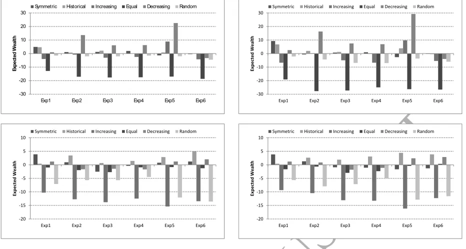
We are first concerned with performance comparison of various investment strategies (obtained by the stochastic and robust portfolio optimization models) in terms of optimal asset allocation of weather futures for HDD and CDD temperature indices on winter and summer periods, based on the US and UK locations. Optimal Asset Allocation: Figure 1 illustrates optimal asset allocations obtained by solving the CVaR optimization model (left) at different targeted wealth and the robust portfolio management models under symmetric (middle) and asymmetric (right) uncertainty sets at varying price of robustness using HDD (top panel) and CDD (middle panel) indices for the US locations as well as HDD (bottom panel) indices for the UK locations. Different colours in Figure 1 represent asset allocations (weights) of various futures contracts on different locations. Note that the optimal asset allocation using the CDD temperature indices based on the UK locations is not presented in this figure since these contracts lead to a conservative strategy suggesting to invest on single location. Recall that, during the summer period, the worst-case temperature is below the threshold level (i.e. average temperature around 18oC) in Britain.
For a fixed price of robustness, the optimal solution of the robust portfolio allocation models under symmetric and asymmetric uncertainty sets determines an investment strategy using weather derivatives on the worst-case temperature error estimation within the corresponding uncertainty set. For the price of robustness that is fixed at zero, the nominal model produces an optimal strategy that invests on single location with the highest return. Generally speaking, Figure 1 shows that the robust portfolios constructed by CDD (HDD) weather derivative contracts using symmetric and asymmetric uncertainty sets display different (same) characteristics. More precisely, we make the following observations:
• The robust decision-making models under symmetric and asymmetric uncertainty sets at fixed price of robustness within a range [0.05, 1.92] provide well-diversified portfolios of HDD weather derivative contracts among different locations in the USA. Note that the northern cities have mean tempera-ture below the reference temperatempera-ture during the winter period. For high price of robustness varying within [1.92, 2.76), the robust strategy (with both symmetric and asymmetric uncertainty sets) is still profitable and diversified. However, the robust model at fixed budget of robustness 2.76 suggests to invest on single location and provides zero profit at the worst-case. This implies that HDD weather derivative contract at the worst-case has no value at certain threshold of budget of robustness (i.e. any allocation gives 0 for the contract).
ACCEPTED MANUSCRIPT
50 100 150 200 250 300
Expected Return
0 0.2 0.4 0.6 0.8
Asset Weights
Price of Robustness
Asset Weights
0 0.05 0.14 0.28 0.5 0.83 1.29 1.92 2.76 0
0.2 0.4 0.6 0.8
Price of Robustness
Asset Weights
0 0.05 0.14 0.28 0.5 0.83 1.29 1.92 2.76 0
0.2 0.4 0.6 0.8
0 50 100 150 200 250
Expected Return
0 0.2 0.4 0.6 0.8 1
Asset Weights
Price of Robustness
Asset Weights
0 0.05 0.14 0.28 0.5 0.83 1.29 1.92 2.76 0
0.2 0.4 0.6 0.8 1
Price of Robustness
Asset Weights
0 0.05 0.14 0.28 0.5 0.83 1.29 1.92 2.76 0
0.2 0.4 0.6 0.8 1
200 210 220 230 240 250 260 270 280
Expected Return
0 0.2 0.4 0.6 0.8 1
Asset Weights
Price of RobUKtness
Asset Weights
0 0.05 0.14 0.28 0.5 0.83 1.29 1.92 2.76 0
0.2 0.4 0.6 0.8 1
Price of RobUKtness
Asset Weights
0 0.05 0.14 0.28 0.5 0.83 1.29 1.92 2.76 0
0.2 0.4 0.6 0.8 1
Figure 1: Optimal asset allocations obtained by the CVaR optimization model (left column), robust optimization with sym-metric (middle column) and asymsym-metric (right column) uncertainty sets using HDD (top row) and CDD (middle row) weather derivatives for the US locations and HDD (bottom row) indices for the UK locations.
the US locations, the robust portfolios constructed using the symmetric (asymmetric) uncertainty set are diversified for the budget of robustness varying within [0.05, 1.92] ([0.05, 0.83]).
• The nominal strategy at zero price of robustness suggests to invest on HDD (CDD) contracts based on Minneapolis (Las Vegas) while the robust strategy with the highest price of robustness, at 2.76, considers HDD (CDD) contracts based on Los Angeles (Portland for symmetric and asymmetric un-certainty sets, respectively). For the UK data set, the nominal strategy also prefers single location of Edinburgh. However, the robust portfolio optimization model (at price of robustness 2.76) provides a well diversified asset allocation strategy among the HDDs based on London, Belfast and Cardiff.
ACCEPTED MANUSCRIPT
whereas the maximum wealth portfolio is constructed by only HDD contract of Southampton.
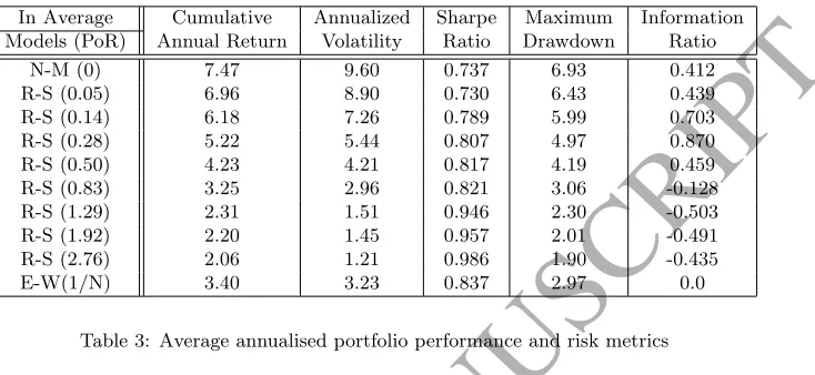
CVaR Investment Decisions: For performance comparison of the CVaR investment strategies ob-tained by weather futures written on HDD temperature indices for the US (left) and UK (right) locations, we construct the simulation-based efficient frontiers as follows. The lowest (Wmin) and the highest (Wmax)
portfolio positions on the efficient frontier are obtained by solving the CVaR (5%) risk minimization prob-lem (ignoring the portfolio wealth constraint) and the wealth maximization probprob-lem (ignoring the risk constraint), respectively. The range [Wmin, Wmax] of minimum and maximum wealth portfolio positions is
discretized by twenty points. At each discrete point on the frontier, we solve the CVaR minimization model (Pcvar) in view of the expected portfolio wealth constraint with fixed target-wealthWtarget ∈(Wmin, Wmax).
As a result, the optimal asset allocations presented in Figure 1 (left column) are obtained. The optimal asset allocation at each discrete point is then evaluated with a sample of 10000 future temperature realizations generated by GH distribution with average errors 0, 0.05, and 0.1 (at fixed unit standard deviation) and standard deviations 0.5, 1, and 1.5 (at fixed zero mean). Figure 2 presents the simulation results in terms of average of the worst 500 evaluated paths in “Expected Wealth” and “Conditional Value at Risk 5%” space. We observe that the CVaR investment strategies produce the highest (lowest) expected wealth as well as
Expected Wealth
0 50 100 150 200 250 300 350
Conditional Value at Risk 5%
-700 -600 -500 -400 -300 -200 -100 0
0 Error 0.05 Error 0.1 Error
Expected Wealth
180 190 200 210 220 230 240 250 260 270
Conditional Value at Risk 5%
-220 -200 -180 -160 -140 -120 -100
0 Error 0.05 Error 0.1 Error
Expected Wealth
-50 -40 -30 -20 -10 0 10 20
Conditional Value at Risk 5%
-260 -240 -220 -200 -180 -160 -140 -120 -100
<=0.5 Error <=1 Error
<=1.5Error
Expected Wealth
9 9.5 10 10.5 11 11.5 12 12.5 13 13.5
Conditional Value at Risk 5%
-75 -70 -65 -60 -55 -50 -45 -40
<=0.5 Error <=1 Error
[image:24.595.77.494.338.645.2]<=1.5Error
Figure 2: Impact of CVaR efficient portfolios using HDD temperature indices for the US (left) and UK (right) locations
ACCEPTED MANUSCRIPT
Performance of Robust Investment Strategies: In order to illustrate performance of the stochastic and robust portfolio allocation models as well as the naive equally weighted investment strategies, we design simulation experiments using two cases (labelled as “Case I” and “Case II”). In Case I, temperature reali-sations are generated by a skewed distribution with mean 1.4 at fixed unit standard deviation whereas Case II uses a skewed distribution of temperature realisations with zero mean and variance 1.9. It is worthwhile to emphasise that Cases I and II basically aim to create unfavourable andfavourableweather conditions to express “weather conditions that were different than expected on average’’ and “weather conditions as we
expected”, respectively. Table 1 summarises the results of simulation experiments using investment strategies
obtained by the stochastic portfolio allocation problem (nominal model, henceforth abbreviated as “N-M”) and the robust optimization models under ellipsoidal uncertainty set (abbreviated as “R-S”) at various budget of robustness (PoR). We also consider an equally weighted portfolio (abbreviated as “E-W (1/N)”) that is constructed by 1/N asset allocations whereN is number of temperature derivatives based on various locations under consideration.
Performance HDD Indices Based on the US Locations HDD Indices Based on the UK Locations Statistics Mean S-Dev Skew Kurt VaR CVaR Mean S-Dev Skew Kurt VaR CVaR
Models Case I: Skewed distribution with high-mean (1.4) and low-variance (1.0)
N-M (0) 67.10 72.03 -0.45 3.00 27.18 16.30 -46.80 116.09 -0.39 3.18 -71.95 -81.06 R-S (0.05) 71.47 65.34 -0.45 2.89 25.86 16.75 -52.42 131.36 -0.41 3.73 -79.45 -84.41 R-S (0.14) 64.26 35.56 -0.46 2.81 33.98 29.40 -50.98 124.65 -0.43 3.42 -73.60 -80.18 R-S (0.28) 66.49 28.43 -0.46 3.03 35.49 29.91 -48.33 120.08 -0.39 3.53 -69.21 -75.62 R-S (0.50) 68.52 20.85 -0.47 3.05 30.52 27.06 -48.57 120.66 -0.41 3.39 -70.35 -75.51 R-S (0.83) 71.76 18.56 -0.45 2.97 25.23 22.47 -47.27 119.90 -0.40 3.29 -69.85 -76.12 R-S (1.29) 77.97 15.15 -0.41 3.02 19.14 18.19 -47.80 118.68 -0.41 3.45 -68.10 -76.05 R-S (1.92) 89.47 15.45 -0.38 3.02 17.48 13.77 -46.96 118.78 -0.38 3.21 -70.90 -75.32 R-S (2.76) 82.95 14.08 -0.37 2.85 -16.88 -22.97 -52.32 129.94 -0.34 3.82 -75.40 -82.06 E-W(1/N) 69.60 14.52 -0.37 2.81 24.48 21.12 -45.86 111.65 -0.36 3.40 -67.75 -71.55
Models Case II: Skewed distribution with zero-mean and high-variance (1.9)
N-M (0) 201.70 94.97 -0.51 2.60 152.98 143.23 64.57 46.40 -0.41 2.79 30.51 23.70 R-S (0.05) 201.34 85.69 -0.53 3.03 155.05 145.79 63.21 25.31 -0.41 2.84 38.06 33.03 R-S (0.14) 170.63 50.05 -0.52 2.62 135.25 128.18 60.57 22.90 -0.40 3.19 36.64 31.85 R-S (0.28) 159.87 38.89 -0.54 2.98 128.68 122.45 57.66 21.68 -0.37 2.97 34.38 29.72 R-S (0.50) 144.80 29.20 -0.54 2.80 117.79 112.38 56.42 21.54 -0.38 3.36 33.21 28.57 R-S (0.83) 130.96 24.27 -0.50 2.79 106.33 101.40 54.82 21.53 -0.35 3.05 31.63 26.99 R-S (1.29) 119.86 21.97 -0.52 2.61 96.43 91.74 53.83 21.54 -0.34 3.05 30.63 25.99 R-S (1.92) 103.36 20.50 -0.50 2.72 80.73 76.20 53.09 21.55 -0.33 3.07 29.88 25.24 R-S (2.76) 92.21 18.32 -0.50 2.96 70.81 66.53 50.73 23.06 -0.32 2.73 26.72 21.92 E-W(1/N) 124.42 19.27 -0.51 2.80 102.08 95.32 53.73 20.25 -0.31 3.08 30.36 25.37
Table 1: Performance comparison of investment strategies with HDD indices based on the US (left) and UK (right) locations.