Consensus of a kind of Dynamical Agents in Network with
Time Delays
Hongwang Yu, Baoshan Zhang
School of Mathematics and Statistic, Nanjing Audit University, Nanjing, China E-mail: [email protected]
Received August 4, 2010; revised September 18, 2010; accepted October 23, 2010
Abstract
This paper investigates the collective behavior of a class of dynamic agents with time delay in transmission networks. It is assumed that the agents are Lyapunov stable distributed on a plane and their location coordi-nates are measured by some remote sensors with certain error and transmitted to their neighbors. The control protocol is designed on the transmitted information by a linear decentralized law. The coordination of dy-namical agents is shown under the condition that the error is small enough. Numerical simulations demon-strate that our theoretical results are valid.
Keywords:Multi-Agent System, Time Delay, Consensus Protocol
1. Introduction
Distributed coordination of network of dynamic agents has attracted a great attention in recent years. Modeling and exploring these coordinated dynamic agents have become an important issue in physics, biophysics, sys-tems biology, applied mathematics, mechanics, computer science and control theory [1-10]. How and when coor-dinated dynamic agents achieve aggregation is one of the interesting topics in the research area. Such problem may also be described as a consensus control problem.
To describe the collective behavior of agents in a large scale network, the agent in the network usually is mod-eled by a very simple mathematical model, which is an approximation of real objects. Saber and Murray [3,4] proposed a systematical framework of consensus prob-lems in networks of dynamic agents. In their work the dynamics of the agent is modelled by a simple scalar continuous-time integrator xu , the convergence analysis is provided in different types of the network topologies. Following the work of [2,3], G. Xie and L. Wang [8] study the case where the dynamics of each agent is second order. In their work, they show that by means of a simple linear control protocol based on the structure of the graph, the dynamical agents will eventu-ally achieve aggregation, i.e., all agents will gradually move into a fixed position of the line, meanwhile their velocities converge to zero.
In networks of the dynamic agents, time delays and sensor error may arise naturally, e.g., because of the moving of the agents, the congestion of the communica-tion channels and the finite transmission speed due to the physical characteristics of the medium transmitting the information. The different protocols with time delays have been investigated [2,4]. And the sensor error or communicated errors are also to be considered in the consensus protocol [9]. It is shown that the collective behavior of dynamical agent will depend on the commu-nicated error and the algebraic characterization of the communicated network topology.
In this paper, we study the consensus of multiagent systems where the dynamics of each agent is second or-der. The agents may represent the vehicles or mobile robots spread over a wild area and they communicate by means of some remote sensors with certain error and time delay. When the agents are moving in a plane, the consensus conditions will depend on the time delay, communicated error and the algebraic characterization of network topology, as well as the dynamical behavior of agents.
2. Preliminaries
By , we denote an undirected graph with an weighted adjacency matrix
( , , )
G V E A
[ ]ij
A a E V V
, where
is the set of nodes, is the set of edges. The node indexes belong to a finite index set
1
{ , , M}
V p p
1, ,
M M .
An edge of G is denoted by . The adjacency elements are defined in following way:
( ,j pi)
ij
e E
ij e p
ij
a
. Moreover, we assume for all 0
ij
a
aii 0 iM .
The set of neighbors of node pi is denoted by
| (
i j
N p V pi,pj)E
Ddiag d .
A diagonal matrix is a degree
matrix of G with . Then the Laplacian of the
, , d
1 M
1
M
i ij
j
d a
weighted graph G is defined as . A graph is called connected if there exists a path between any two distinct vertices of the graph.
L D A
An important fact of L is that all the row sums are zero, therefore, is an eigenvector of L associ-ated with zero eigenvalue. Moreover, the graph G is connected if and only if its Laplacian L is satisfied rank(L) = M− 1 and all eigenvalues of L are of positive real numbers except that only one eigenvalue is zero [2].
1 1, ,1TM
Consider a network of dynamical agents defined by a graph . The node set V consists of dy-namical agents
( , , ) G V E A
,
i
P iM . Let xi ( ,xi1 xi2)TR2 P
be the coordinate of dynamical agent i, then the dynamics of pi are identical and described as follows.
i i
i i i i
i i
i
x v
m v Kv u
x
y F
v
(1)
where xi is indicates the location vector of agent i
in the plane, represents its velocity vector p
1 2
( , )T
i i i v v v
of the ith agent, mi is its mass and is
11 12 21 22
k k
K
k k
a dynamical feedback matrix of the agent. F is an obser-vation matrix of the agent by some remote sensor. In what follows we simply assume that mi1 and pixi.
Let which means that the location informa-tion of the ith agent is only measured by some remote sensor and is transmitted to its neighbors through the network. The matrix C is assumed to be the form
[ 0]
F C
1 1
i
i
C
. The parameter i indicates that the
network communicated error or the coordinates used for sensor could be different from that of the agents.
For the dynamic agent (1) in network we have follow-ing assumption.
Assumption 1. The dynamics (1) is Lyapunov stable when it disconnected with its neighbors, meaning that the dynamical agent as an autonomous will gradually stop by moving a finite distance for any non-zero initial velocity. We shall give the conditions, under which the network of dynamical agents (1) achieve asymptotical consensus meaning that there exists a fixed position (equilibrium)
such that for
2
R
x iM
2 1
lim ( ) lim ( ) 0
i t
i t
x t x
v t
(2)
Due to time-delay in communicated network, the con-trol protocol of the dynamical agent i is a neighbor-
based linear control law in the form that p
( ( ( )) ( ( )))
j i
i ij j ij i ij
p N
u a y t t y t t
(3)where i is the set of neighbors of agent i and ijare adjacency elements of A. The
N p
a ij( ) 0t , denoting
the communication transmission time-delay from agent
j
p to agent i. In this paper, we discuss the consensus of dynamical agent under the condition of the communi-cated error and the time delay. We focus on the simplest possible case where the time-delays in all channels are equal to
p
and the communicated errors are equal to .
Remark 1. If we choose 0 and k11k22 k, 12 21 0
k k , then the two-dimension agent systems (1) with the control protocol (3) can be decoupled into two identical linear systems and it was discussed by some literatures with or without time delays( such as [8,9]).
3. Consensus of Dynamic Agents
We denote the initial locations and the initial velocities of the agents by
1
(0) ( (0)T T(0))
M
x x x T (0) ( (0)1 (0))
T T
M
v v v
, T
respectively. Under control protocol (3) with ij( )t , the dynamical equation of agent pi is written by
( ) ( ) ( ( ) ( ))
j i
i i ij j i
p N
t A t B a t t
where ( ) ( ( ),T T( )) , i t x t v ti i
T iM
2 2 2 2 2 2
0 0
I A
K
, . (4)
2 2 2 2 2 2 2 2
0 0
0 B
I
T
Furthermore, let 1 , then the
dynamic network is of the following form ( ) ( T( ), , T( ))
M
t t t
1 2
( )t ( )t (t )
(5) where
1 IM A, 2 L B
And L is the Laplacian associated with the connected graph G. Because (5) is a standard linear time-delay dy-namical systems, its stability analysis is equivalent to analyzing the eigenvalues and eigenvectors of matrix
. 1 2
Lemma 1. The matrix 1 2 has two
eigen-vectors associated with zero eigenvalue. Let e
e
, be the left and right eigenvectors (denoted by matrices) of matrix associated with zero eigenvalue, respectively. Then
2 2
1 1 T
T M K I M , 1 2 2 1 1 0 M K M
(7)
and I2 2 , where 1
1, ,1
T M
M R .
Proof It is well known that (refer to [2,11]) the graph is connected if and only if its Laplacian satisfies that rank(L) = M− 1. Moreover,
is an eigenvector of L associated with zero eigenvalue. Then, there is only one zero eigenvalue of L, all the other ones are positive and real. By the definition of (6) and
, one has ( , , )
G V E A
1 e
1 1, ,1T
M
2
2 2 1 2 2 2 2 2 2 2
2 2
2 2 2 2 2 2
2 2 2 2 4 2 1 1 0 1 1 0 0 0 1 1 0 0 M M M T T M T T M
K I e
M
I
I K I
K M
e L e L K I
I M Thus, 2 2 1 1 T T M K I M
represents the two left eigenvectors of .
Similarly, it is easy to check 04M2, which
im-plies that
1
2 2 1 1 0 M K M
represents two left-
eigenvectors of . And it is holds that I2 2 . Theorem 1 If the dynamical feedback matrix K in dynamical agent (1) satisfies Assumption 1, i in
the C of (1) and the time delays ij( )t in (3)
satis-fies
min max
(8) with
min 2 ( 2 2)
abc d
e a b
, max 2 ( 2 2)
abc d
e a b
(9)
where , , ,
and
21 12
ak k
2 2
( ) 4e a(
11 22
b k k 2) 2 b b c
11 22 12 21
ck k k k
d abc M denotes
the biggest eigenvalue of matrix L, then all of the
eigen-values of 1 e 2
0
defined in (6) are of negative real parts except for only two zero eigenvalues.
Proof As the graph G is connected, one denotes the eigenvalues of L by 12M . There
exists an orthogonal matrix W such that
1 2
{ , , , M}
iag T
W LW d
4 4 4 4 4 4 4 4 ( ) ( ) 0 0 M T T
W I W
W I I
A e B
. One can verify the following formulae.
4 4
4 4
1 4 4 4 4
2 4 4
4 4 ( ) ( )( 0 0 0 0 M I
A e L B W I
A e B
)
A e B
Then the dynamical behavior of the network (1) is char-acterized by the eigenvalues of A ie B, i M
.
First we discuss the block with 10. By
Assump-tion 1, one has
11 22 0,
k k k k12 21k k11 22 (10) and rank(A1e B )2
1 2 0, (
s s
, its four eigenvalues satisfy
3) 0, ( ) 04
Re s Re s
For i0, one has
2 2 2
0 i i I A B C e e k
. As
( )
rank C 2 , then . Therefore,
1 2
(Aie B)
rank
4
e
has only two zero eigenvalues. Consider the characteristic polynomial of A ie B
for iM .
11 12 21 22 4 3 2
1 2 3 4
( ) ( ( ))
0 1 0
0 0
i
A B i
i i
i i
s det sI A B
s
s 1
s k k
k s k
e
e e
e s
e
a s a s a s a where
1 11 22 2 11 22 12 21
3 21 12 11 22 2 2 2
4
, 2
( ) ( )], ( , [ 1 ) i i i e e
a k k a k k k k
a k k
e k k a (11)
Construct the Routh array of AiB( )s
with 1 2 3 2 2 2
1 2 1 4
1
, i
a a a
b b d a e
a
(1 ),
2 2 1 3 1 2 1 2 3 3 1 4 1
1 1 1
. b a a b a a a a a a c
b a b
By the criterion, for stability it is necessary that 1 1 1 1 . Therefore, the dynamical network is stable if and only if the following inequalities hold
RouthHurwith 0, 0,
a b c 0,d 0
1 4 1 2 3
2 2 1 2 3 3 1 4
0 0 0 0 a a
a a a
a a a a a a
(12)
By (10) and (11), it is obvious that the first and second inequalities in (12) hold, and one may easily verify that the third inequality in (12) holds only if the fourth ine-qualities holds. Then
2 2 1 2 3 3 1 4
11 22 11 22 12 21 21 12
2 2 2 2 2
11 22 11 22 21 12
{( ) ( ) [ ( )
( )]} i i [( ) (
a a a a a a
k k k k k k k k
k k e e k k k k
) ] 2
So the fourth inequality in (12) can be rewritten as the following form.
2 ( 2 2) 0
i i i
b cabc e a b (13)
where 21 12 , , .
From it, one may obtain
ak k b k11k22 ck k11 22k k12 21
2 2 2 2
2 ( ) 2 (
i i
i
i i
abc d abc d
e a b e a b
)
2
where . Under the case,
the matrix i
2 2 2
( ) 4 ( )
i i
d abc e a b b c
AeB is Hurwith. Then it is obvious that the matriies A ie B
are Hurwith
for all under the condition of (8) and (9). There-fore, all of the eigenvalues of the matrix 1 2 defined in (6) are of negative real parts except for only two zero eigenvalues.
2, i ,M
e
Theorem 2 Under conditions of Theorem 1, the con-trol protocol (3) globally and asymptotically achieves the collective behavior of the dynamic agents.
Proof Under conditions of Theorem 1, all of the ei-genvalues of the matrix 1 2 defined in (6) are of negative real parts except for only two zero eigen-values. By
e
4 1 4
, , , ) 4 4
1 2
: ( , M M
R
M M one
denotes right-eigenvectors of associated with eigen-values 1, ,2 ,2M
respectively.
It holds that , 2 2 1 ,
1
diag 0 , , , J JM
J denotes the Jordan form of two order associated with the eigenvalues 1 and 2. Ji denotes the Jordanform of four order associated with the eigenvalues
4 3i , 4 2i , 4 1i
and 4i for all i2, , M .
4 1, 4 )
Let 1 : ( T T, , 4 4
1 , 2
M M R
M M
T T T
,
where i;i4M are 4M row left-eigenvectors of correspondingly. Then it is holds that .
4 1
(
Re R
As 0 Re(3) Re(4) M ) e( 4M)
2 (4 2) 4 2) (4 2)
M M
) 2 (
0
0 M 0 M
,
one has 2 2
(4 2
I
lim Jt te
2 (4 2) (4 2) (4 2
0 0 0 M M M and 2 2
4 2) 2 M )
(
I
lim ( )
texp t
Let ( 1 2)and
2 1
, one has li
tmexp t( ) .
Due to the fact that 1
4 4
· · I MM
, and
satisfy the property I2 2 .
1 2 2 2 2 2 ( 0 exp k 2 (0) · ( · (0) k I 1 2 2lim ( ) lim ) (0)
1 0) 1 0 0 t t M M M M t t M I k M 1 1 1 1
Therefore, (0) 1 (
i xj k v
, 2, , }M
1
1
lim ( { [M j 0)]}
t j x t M )
0, and it is obvious thatlim ( )i {1
tv t i
This implies the protocol (3) globally asymptotically achieves the collective behavior of the dynamic agents.
Corollary 1 The dynamical feedback matrix K is chosen to be k12 k21k1 and 11 22 2, then the control protocol (3) globally and asymptotically achieves the collective behavior of the dynamic agents if the time
k k k
satisfy
2 2 2 1
2
delays lnk k
.
Proof It is easy to verify according to the proof of Theorem 1 and Theorem 2. Under Assumption 1, one has
12 21 11 22
k k k k . Thus, one finds that and it further implies that min
0
c
0
and max 0 in (9) for bounded
time delay. Thus we have the following result.
Corollary 2 The dynamical agents achieve collective behavior if the network communicated error is suf-ficient small for the bounded time delays.
4. Simulations
Con-sider five dynamic agents under network described in Figure 1.
We can obtain the Laplacian matrix L of the graph G of Figure 1 and its eigenvalues are 1 0 , 23
1(7 13)
2 , 4 5
1(7 13)
2
, 64.
We consider that the dynamic agent (1) in the network has 1 0.1 ,
0.2 1 k
0.1 in the observation matrix C and the time delay 0.1 in (3). Thus, it is
stable and satisfies Assumption 1. One can get
Lyapunov
0.1
a ,
, ,
2
c0.98
b 12.1324and the 0.1 belongs
to the range of parameters, i.e.,
min 0.2125 0.2764 max
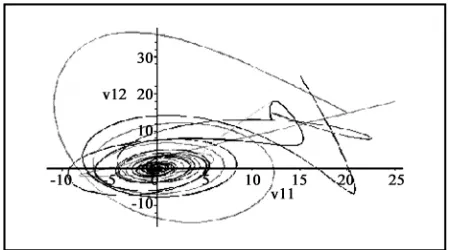
When a control protocol (3) is applied into the agents in network, the collective behavior of dynamic agents takes place according to our result. Figures 2-3 give simulation results of the collective behavior of the agents while their velocities.
5. Conclusion
In this paper, we discuss the collective behavior of dy-namical agents in network which associated with a graph
[image:5.595.311.537.77.202.2]Figure 1. An undirected graph G with M = 6 nodes.
Figure 2. State trajectories of the agents in G.
Figure 3. Velocity trajectories of the agents in G.
G. It is assumed that the agents are Lyapunov stable dis-tributed on a plane and their location coordinates are measured by some remote sensor with certain error and transmitted to its neighbors. Based on the transmitted information with time-delay, the control protocol is de-signed as a linear decentralized law. The coordination of dynamical agents is shown under the condition that the error is small enough. There is a tradeoff between ro-bustness of a protocol to time-delays and the sensor er-ror.
6. Acknowledgement
This work is supported by the Nanjing Audit University Fund (No. 20720035).
7. References
[1] A. Jadbabaie, J. Lin and S. A. Morse, “Coordination of Groups of Mobile Autonomous Agents Using Nearest Neighbor Rules,” IEEE Transactions on Automatic Con-trol, Vol. 48, No. 6, June 2003, pp. 988-1000.
[2] R. O. Saber and R. M. Murray, “Consensus Problems in Networks of Agents with Switching Topology and Time- Delays,” IEEE Transactions on Automatic Control, Vol. 49, No. 9, September 2004, pp. 1520-1533.
[3] R. O. Saber, J. A. Fax and R. M. Murray, “Consensus and Cooperation in Networked Multiagent Systems,” Pro-ceedings of the IEEE, Vol. 95, No. 1, January 2007, pp.
215-240.
[4] P. Lin and Y. Jia, “Average Consensus in Networks of Multi-Agents with Both Switching Topology and Cou-pling Time-Delay,” Physica A: Statistical Mechanics and Its Applications, Vol. 387, No. 1, January 2008, pp.
303-313.
[5] Y. Liu and K. M. Passino, “Stable Social Foraging Swarms in a Noisy Environment,” IEEE Transactions on Automatic Control, Vol. 49, No. 1, 2004, pp. 30-44. [6] V. Gazi and K. M. Passion, “Stability Analysis of Social
[image:5.595.64.541.412.734.2]Agents in Directed Network,” Proceedings of the 26th Chinese Control Conference, 2007, pp. 557-561.
[8] G. Xie and L. Wang, “Consensus Control for a Class of Networks of Dynamic Agents,” International Journal of Robust and Nonlinear Control, Vol. 16, 2006, pp. 1-16.
[9] L. Yang, H. Yu and Y. Zheng, “Aggregation of Dynamical
Agents in Network,” 7th World Congress on Intelligent Control and Automation, June 2008, pp. 6348-6352.
[10] N. Biggs and Algebraic, “Graph Theory,” Cambridge University Press, Cambridge, 1994.