Thermodynamics of the classical spin ice model with nearest neighbour interactions using the Wang Landau algorithm

DOI:10.1140/epjb/e2016-60781-7

Regular Article

P

HYSICAL

J

OURNAL

B

Thermodynamics of the classical spin-ice model with nearest

neighbour interactions using the Wang-Landau algorithm

Maria V. Ferreyra1,2, Gaston Giordano3, Rodolfo A. Borzi1, Joseph J. Betouras4, and Santiago A. Grigera1,5,a

1 _{Instituto de F´ısica de L´ıquidos y Sistemas Biol´ogicos (IFLySIB), UNLP-CONICET, 1900 La Plata, Argentina} 2 _{Facultad de Ciencias Exactas y Naturales, Universidad Nacional de La Pampa, 6300 Santa Rosa, Argentina}

3 _{Departamento de F´ısica, Facultad de Ciencias Exactas, Universidad Nacional de La Plata, 1900 La Plata, Argentina} 4 _{Department of Physics, Loughborough University, Loughborough LE11 3TU, UK}

5 _{School of Physics and Astronomy, University of St Andrews, St Andrews, KY16 9SS, UK}

Received 1st October 2015 / Received in final form 10 December 2015 Published online 22 February 2016

c

The Author(s) 2016. This article is published with open access atSpringerlink.com

Abstract. In this article we study the classical nearest-neighbour spin-ice model (nnSI) by means of Monte Carlo simulations, using the Wang-Landau algorithm. The nnSI describes several of the salient features of the spin-ice materials. Despite its simplicity it exhibits a remarkably rich behaviour. The model has been studied using a variety of techniques, thus it serves as an ideal benchmark to test the capabilities of the Wang Landau algorithm in magnetically frustrated systems. We study in detail the residual entropy of the nnSI and, by introducing an applied magnetic field in two different crystallographic directions ([111] and [100]), we explore the physics of the kagome-ice phase, the transition to full polarisation, and the three dimensional Kasteleyn transition. In the latter case, we discuss how additional constraints can be added to the Hamiltonian, by taking into account a selective choice of states in the partition function and, then, show how this choice leads to the realization of the ideal Kasteleyn transition in the system.

1 Introduction

In magnetism, when a spin cannot fully minimise its interactions with its neighbours, the system is called “frustrated”. This situation can arise under a number of different circumstances such as bond disorder, further neighbour interactions and lattice geometry. Geometri-cally frustrated magnets are the cleanest and better con-trolled in experimental systems. Frustration precludes the formation of simple ordered ground states. Rather, it typ-ically leads to a degenerate manifold of ground states which are unstable to small perturbations. Frustrated sys-tems exhibit a rich variety of behaviour, including order by disorder, fractionalisation and magnetic analogues of solids, liquids, glasses, ice, quantum liquids and Bose con-densation. They represent ideal model systems for the study of generic concepts relevant to collective phenom-ena, where simple classical Hamiltonians can give rise to a wealth of different phenomena [1–3]. All this make ge-ometrically frustrated systems the focus of attention of both theoretical and experimental research, making for ideal test-grounds for numerical techniques.

Among the developments in classical simulation tech-niques, the Wang-Landau algorithm (WLA) has stood out

a _{e-mail:[email protected]}

ferromagnetically at nearest neighbours – exhibits an ex-tremely rich behaviour. The degeneracy of the zero field ground state grows exponentially with the system size and has construction rules analogous to those of protons in water ice. By applying an external magnetic field it is possible to find a metamagnetic transition or to tune into an effective two dimensional model (the kagome-ice, also with extensive residual entropy) and to find two- and three-dimensional Kasteleyn transitions. The physics of this model system has been well studied using a variety of techniques [9–13], and thus serves as an ideal benchmark to test the capabilities of the WL algorithm in this type of systems. Beyond that, the WLA provides new ther-modynamic results that have not been obtained by other methods, such as the free energy as a function of the order parameter, which, to our knowledge, has been calculated for a Kasteleyn transition for a first time.

The structure of this article is as follows. In the next section we give a brief discussion of the model and the sim-ulation technique for completeness. In Section 3, we study the model at zero applied field, calculate the residual en-tropy and compare it with different existing estimates us-ing the WLA technique. In the same section, we study the system under field applied along [111], and explore the entropy of the kagome-ice state, as well as the entropy peak that rises when this state is destroyed by increasing the temperature. Finally, we study the case of field ap-plied along [100], and do a characterisation of the three dimensional Kasteleyn transition into the fully polarised state.

2 Methods

2.1 Wang-Landau algorithm

In 2001, Wang and Landau introduced an algorithm to estimate the density of states of a system by performing a random walk in energy space [4,5]. This method is closely related to “umbrella sampling” techniques [14] and multi-canonical Monte Carlo [15]. The algorithm provides a very good estimate of the DoS of the system over a bounded region of the energy spectrum. The DoS can be calculated as a function of the energy, if one works in the canon-ical ensemble, but also as a function of other variables like pressure or magnetisation if one is interested in other ensembles such as the isothermal-isobaric or its magnetic equivalent (as we will use in Sects. 3.2 and 3.3). In this section we describe the procedure for one variable, which is then straightforwardly extended to the case of several variables.

The algorithm requires the knowledge of the Hamiltonian of the system and a method to sample con-figurations− in our case it is simply random single spin flips. The starting point is an arbitrary initial config-uration with energy E0. Initially, the DoS is taken as

homogeneous:g(E) = 1 for allE. One step of the calcula-tion consists then in choosing new random configuracalcula-tion, calculating its energy E1, and accepting it or discarding

it with probability

p(E0→E1) = min

1,g(E0) g(E1)

. (1)

At each step, the histogram H(E) and the DoS g(E) of the final configuration are modified according tog(E)→ g(E)f andH(E)→H(E) + 1. Initially the modification factor f for g(E) is taken from a larger value (usually, f0 = e1) which is then reduced as the algorithm pro-gresses. The rule by which the modification factor f_i is reduced is an important choice that conditions the accu-racy of the DoS and speed at which the process converges. In principle, one can choose any function that tends mono-tonically to one, and stop the process once f reaches a given value. In the original work, Wang and Landau pro-pose the rule f_k+1 =√fk, but other choices are possible which give faster convergence. In particular, Belardinelli and Pereyra (BP) [16] proposed an alternative method with improved convergence times, in which the modifi-cation factor is eventually scaled as the inverse of the Monte Carlo time, t. For this work we have adopted the BP algorithm.

In our case, within one Monte Carlo step this proce-dure was repeated with single spin flips until the spin of each site had been chosen to change at least once on aver-age. In practice, the quantity lng(E)→lng(E) + lnf is used for simplicity (hence the choicef0=e). Notice that

this procedure guarantees that the random exploration in phase space will not jam at local minima: each time the transition to the new state is not accepted, the DoS of the initial state is increased and thus the probability of ac-cepting any future transition, which will be proportional tog(E0), is also increased. The detailed balance condition is satisfied to within lnf accuracy.

During this random walk through phase space, the histogram is accumulated and checked periodically. WhenH(E) becomesflat, the histogram is reset, and the next random walk begins with a finer modification fac-tor f1. The criterion of flatness varies according the size

and complexity of the system. Usually, the criterion used for flatness is that every entry inH(E) is not smaller than a percentage of the average histogram for allE.

The final result is a relative DoS. To calculate the ab-solute values one needs some additional information, e.g. a known point in the DoS – in our case the high temper-ature value of the DoS tends to 2, or the knowledge of the integral of the DoS – in our case 2N. Once the DoS of the system is known, it is straightforward to calculate the thermodynamic quantities in the canonical ensemble: for example, from

Z =

i

g(E_i)e−Ei/kBT_,

the free energy can be written as:

F(T) =−kTlogZ,

the internal energy

U(T) = 1 Z

E

E/k(K/Dy ion)

ln(

)

g(E)

0 200 400 600 800

-1 0 1 2 3 4

Fig. 1.Natural logarithm of the density of states of the nnSI model for a system size L= 4. Its shape is characteristically asymmetric with high degeneracy of the ground state. The inset shows an schematic view of the pyrochlore lattice.

the entropy

S(T) = U(T)−F(T)

T ,

and the specific heat, using the usual linear fluctuation relation,

C(T) =E

2

T −(E_T)2

T2 .

2.2 Spin ice

The nnSI Hamiltonian under an external magnetic field reads:

H =Jeff

ij

Si·Sj−gμB

i

H·Si, (2)

where theS_i are Ising spins situated at the corners of a pyrochlore lattice (see inset of Fig.1), H is the external magnetic field,gthe gyromagnetic ratio andJeff is the

ef-fective exchange interaction which is taken to be positive. The model is applicable to a certain class of materials, of which the most notable examples are Dy2Ti2O7 and Ho2Ti2O7. In these materials, the magnetic ions sit at the corners of a pyrochlore lattice and are constrained by the crystalline field to point along the local 111 quantiza-tion axes (i.e. to or from the centre of the tetrahedra). The nnSI model provides a very good description of these materials between 0.2 K and 10 K [17]. The main differ-ence arises from the fact that in the materials, in addition to the exchange interaction – which is antiferromagnetic – there is a large long range dipolar interaction. If the latter is truncated beyond the nearest-neighbour spins, Jeff is effectively ferromagnetic [18].

The ground state of the nnSI scales exponentially with system size and obeys the local construction rule that within any tetrahedra, two of its spins should point in-wards, and two outwards [17,18]. This rule is called the

“ice-rule” given its analogy to the Bernal and Fowler rules for protons in water-ice [19] and is the origin of the epithet “spin-ice” given to these models. The exponential degen-eracy of this ground state leads to an extensive residual entropy at zero temperature.

We analysed the nnSI model using the WLA with both the original implementation and the one proposed by Be-lardinelli and Pereyra. In order to reach larger lattices we also performed simulations dividing the energy range in multiple regions. To normalize the DoS, we generally used the condition that there are only two states with max-imum energy (the “all-in” and “all-out” configurations). The comparison between several runs performed with dif-ferent seeds, or different normalisation, allowed us to esti-mate the errors on the residual entropy for different sizes. We explored the configuration space through random sin-gle spin-flip moves. In addition, we used a conventional cu-bic cell for the pyrochlore lattice, which contains 16 spins, and simulated systems withL×L×Lcells, withLranging from 1 to 8 (16 to 8192 spins). The DoS was estimated as a function of energy with the modification factor changing fromf0=e1 toffinal= exp(10−9).

For the results of Section 3.1 we used the single-variable WLA, while for Sections 3.2 and 3.3 we accu-mulated the DoS as a function of both the energy and the magnetisation in the direction of the applied magnetic field. In this latter case, the thermodynamic quantities are calculated using a partition function which is summed in the energy and in a variable conjugate to the magnetic field, in this way the derivatives of Z provide informa-tion about the average magnetisainforma-tion. We have chosen J = 1.11 K in order to match the effective nn exchange constant for Dy2Ti2O7.

3 Results

3.1 Spin-ice with no applied external field: residual entropy

As a first step we analysed the nnSI model with no applied external field (H = 0), in particular, we were interested in the behaviour of the specific heat and the entropy. In Figure1it is shown the logarithm of the DoS of the nnSI model for a system sizeL= 4. Its shape, in contrast with the highly symmetrical DoS of the ferromagnetic Ising model (see e.g. Ref. [5]), is characteristically asymmetric, starting from a high value at the lowest energy, a direct measure of the high degeneracy of the ground state.

Fig. 2.Specific heat (green) and entropy (red) vs. temperature for system size L = 4, calculated from the density of states (DoS) with parameters set for Dy2Ti2O7. The figure shows the expected Schottky-like peak in the specific heat, marking the onset of spin-ice correlations. The entropy does not vanish as the temperature is lowered towards T = 0 but shows the residual value characteristic of all ice models.

Rln 2 ≈5.76 J/mol K, indicating that the system is be-having as an uncorrelated paramagnet. As the tempera-ture is lowered the entropy is reduced until it reaches a residual valueS0 close to 1.7 J/mol K.

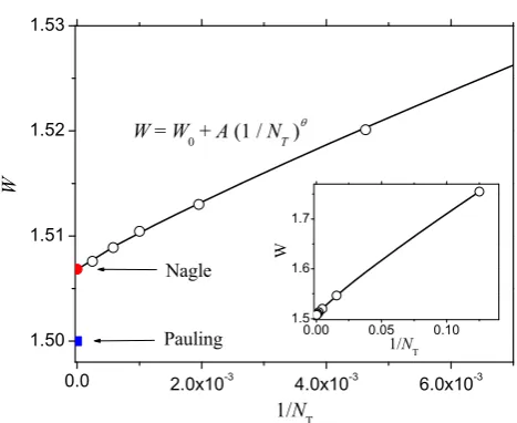
The residual entropy is a characteristic feature of ice models; in real spin-ice materials, such as Dy2Ti2O7 or Ho2Ti2O7it is expected that the degeneracy of the spin-ice manifold will be lifted by additional interactions – chiefly the dipolar interaction – and that the system at T = 0 will be ordered [21,22]. In the nnSI model, how-ever, the construction rules are strictly those of Bernal and Fowler, and one expects to find an exponentially de-generate state with the same extensive residual entropy of the three dimensional ice models. The determination of the value of this entropy has a long history, starting with Linus Pauling’s famous estimate in 1935 [23]. S0 can be written as:

S0=klnWN (3)

where kis Boltzmann’s constant and W_N =WNT _{is the}

number of microstates that form the ground state of the system, withN_T the number of tetrahedra. Pauling’s esti-mate givesW = 3/2, which translated to the entropy per mole givesS0=R/2 ln 3/2≈1.68 J/molK, in reasonable

agreement with the results of Figure2.

Pauling’s estimate neglects correlation effects (in the form of loops) and it can be shown that it is a lower bound on the trueS0[24]. While an exact solution exist for

two dimensional ice models [25], this is not true for three dimensions. Currently the best estimate of the entropy for three dimensional ice is that due to Nagle [26], who, building on work by Di Marzio and Stillinger [27], used a series expansion method to derive the estimate

WNagle= 1.50685(15). (4)

Fig. 3.The number of microstates of the ground state,W, as a function of the inverse of the number of tetrahedra 1/NT. As expected, the residual entropy decreases as the system size is increased. Shown for reference are the thermodynamic value of

W from Pauling’s estimate (blue square) and from Nagle’s cal-culation (red circle). The line is a fit according to equation (5). The inset shows the full range of the fit (fromL= 1 toL= 8).

Corrections to Pauling’s entropy have been studied in the specific case of the pyrochlore lattice, such as the Numer-ical Linked Cluster expansion of reference [28]. The most accurate calculation ofS0for the nnSI model in the litera-ture comes from the integration of energy and magnetisa-tion data obtained by loop Monte Carlo simulamagnetisa-tions [10] and gives W_I = 1.5071(3), very close to Nagle’s result. The WLA provides a direct determination of the entropy without the need of integrating the specific heat and speci-fying additional constants, and is thus ideally suited for an accurate determination of the residual entropy of the nnSI model. A variant of the WLA has been successfully applied to determine the residual entropy of two simple nearest neighbours ice models in three dimensional hexagonal lat-tices: the six-state H2O molecule model and the two-state

H-bond model [29]. A similar method is applied to nnSI. We have calculated the DoS for lattice sizes L = 1 to 8 which correspond toN_T = 8 to 4096 tetrahedra, and from those determinedW for the ground state. Figure3shows W as a function of the inverse of the number of tetrahe-dra 1/N_T. We have used two different criteria to normalise the DoS: in one case we used a known density for a given state (the highest energy state) and in the other we used the sum of all states (2N in our system). The differences in W given by the different criteria of normalisation, or that obtained in independent runs using a different set of random numbers, are smaller than the size of the symbols in the figure.

Figure3shows that, as expected, the residual entropy decreases as the system size is increased. In order to obtain the thermodynamic value ofW we perform a least-squares fit this data to the form

W(x) =W_∞+a1

1 N_T

θ

Fig. 4.Logarithm of the DoS as a function ofEandM along [111] calculated for a system of size L = 3. The figure also shows the projection of the DoS over theM-E plane.

From this fit we obtain W_∞ = 1.50682(9), with a1 =

1.557(9) and θ= 0.883(3). The sub-linear value ofθis an indication of bond correlations in the ground-state mani-fold [29,30]. Our value forWin the thermodynamic limit is perfectly consistent with the results by Nagle (see Eq. (4)) and by previous calculations [10,29].

3.2 Spin-ice: field along [111]

A remarkable feature of the nnSI model is that an exter-nal magnetic field can tune the system into regions of dif-ferent physics. Two notable cases happen when the field is oriented (i) along the crystallographic [111] direction, which will be described in this subsection, and (ii) along [100], which will be described in the following subsection. To describe the effects of an applied external field in the WLA, on one hand the Zeeman term must be included in the Hamiltonian (the second term in Eq. (2)) and, on the other hand, it is more convenient to calculate the DoS as a function of two indices: energy and magnetisationM, the latter being the quantity conjugate to the field. In this way is it possible to work in the magnetic equivalent of the isothermal-isobaric ensemble and obtain directly from the doubly summed partition function the Gibbs free en-ergy G(H, T) and the mean value of M. The disadvan-tage of this approach is that it is too expensive in calcula-tion resources and, therefore, the calculacalcula-tions are usually constrained on smaller system sizes.

Figure4shows the logarithm of the DoS as a function of E and M along [111] calculated for a system of size L= 3. As expected, the DoS is still asymmetric along the Edirection (cf. Fig.1) and symmetric in theM axis. The figure also shows the projection of the DoS over theM-E plane, which takes the shape of a pentagon. In this projec-tion one can see that while the highest energy state cor-responds to M = 0 the ground state manifold comprises a range of magnetisation values; forH [111] this range goes from−3.33 to 3.33μ_B which is the highest value of the magnetisation that can be obtained along [111] with-out breaking the ice rules.

In references [10,11] the case of the external field along [111] has been studied for the nnSI model both

analyti-Fig. 5. Magnetization vs. field along the [111] axis for

L= 3 and different values of temperature. The magnetiza-tion curves present two well defined plateaux. The first one, at 3.33μB/Dy ion, correspond to a state where all apical spins are aligned with the field (the kagome-ice state). The second plateau, at 5μB/Dy ion, corresponds to the state of maximal spin projection along [111]. The inset shows the logarithm of the density of states as a function of the magnetisation at a fixed energyE(E/k_B= 0.1 K above the ground state).

m = 3.33μ_B per Dysprosium ion, which is easily calcu-lated by taking into account the ice-rules and the differ-ent projections of the spins in the kagome and triangu-lar planes1. If the field is increased further, it eventually overcomes the exchange interaction and the system goes through a metamagnetic increase of the magnetisation (at around 1 T in Fig.5) to a fully polarised state where all spins maximise their projection with the magnetic field (m = 5μ_B/Dy ion). In the nnSI model this sudden in-crease is merely a crossover and its width is strongly tem-perature dependent. If the dipolar interactions are added to the model, the metamagnetism becomes a first order transition [31].

As mentioned before, the ice-rules in the KI phase do not fully constrain the system and allow for an exponen-tially large number of possible configurations. In this case it is possible to obtain an exact solution for the residual entropy due to a mapping from the KI into dimers in a honeycomb lattice [11,32]. This mapping allows the study of the effects of slightly misaligned fields, which lead to a two-dimensional Kasteleyn transition (see Ref. [11]), as well as the transition to the fully polarised state, which can be interpreted as a dimer-monomer transition and is expected to be accompanied with a peak in the entropy as a function of field [10].

In conventional MC simulations, the calculation of the field dependent entropy usually includes the integration of the specific heat as a function of temperature, with the integration constant for each field point determined by the value at an appropriate fixed point. In the case of the WLA this calculation is straightforward from the known g(E, M) and requires no further input.

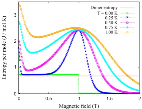
We have calculated the entropy as a function of field along [111] for different temperatures (see Fig.6) from the DoS forL= 3. The green curve shows the T = 0 result: here the entropy jumps from its zero field value (the 3D ice-entropy) to the KI value (close to 0.7 J/mol K) and at higher fields (around 1 T) jumps down to zero as the system becomes fully polarised. The red line is the exact value for the KI entropy (S0= 0.6715 J/mol K) as

calcu-lated in references [11,32]. The slight discrepancy between the calculatedS0and the exact result is due to finite size effects. It is worth pointing out that despite its name and the fact that the coordination number of the lattice is 4, the KI is not sensu stricto an ice-type model2 and thus its residual entropy is smaller: W_KI = 1.175, compared

1 _{In the KI configuration, the apical spin is fully aligned}

with the field, thus contributingμ to the magnetisation. The spins in the kagome plane have a 1/3 projection into [111]; of them, two point with this component towards the field and one points opposite, the net contribution is thus 1/3 μ. The total magnetisation per spin is then: (1 + 1/3)/4μ≈3.33μB.

2 _{Ice-models are defined on lattices of coordination number 4}

and due to the ice-rules have a degeneracy of six states for a single independent plaquette. In the kagome-ice, there are only three possible states per plaquette. Even its extension, the kagome spin-ice (see Ref. [33]) is only ice-like, in the sense that the vertices (the centres of the triangles) form a lattice of coordination number 3.

Dimer entropy T = 0.00 K 0.25 K 0.50 K 0.75 K 1.00 K

Magnetic field (T)

Entropy per mole (J / mol K)

0 0.5 1 1.5 2

0 1 2 3

Fig. 6.Entropy vs. magnetic field forL= 3 and for different values of the temperature. The T = 0 curve shows how the entropy is reduced to zero through two steps: a first one into the KI state, and a second one (at about 1 T) when the sys-tem becomes fully polarised. At higher sys-temperatures the most noticeable feature is a giant entropy peak at the polarisation transition (see text).

toW2D = (4/3)3/2= 1.539. . . At high temperatures, the most notable feature is the appearance of a giant peak in the entropy, which at low temperatures (below 0.7 K) is larger than the residual entropy, and becomes a peak of infinitesimal width at T = 0 (not seen in the figure due to the discretisation of the data). It might seem counter-intuitive that the application of an ordering field might result in an increase of the entropy. This can be explained simply, with the aid of the dimer mapping, as coming from the crossing of an extensive number of energy levels, corre-sponding to different numbers of monomer defects, which have macroscopic entropies (see Ref. [10]). In real materi-als though, this feature of the nnSI model, which has po-tential applications for magnetocaloric manipulations, is almost completely suppressed by additional interactions.

3.3 Spin-ice: field along [100]

A case of particular interest arises when an external field is applied in the [100] direction. In this case, contrary to the previous one, the fully saturated state belongs to the zero field ground-state manifold, that is, it satisfies the ice-rules. At low temperatures (kT Jeff) and for any value of the magnetic field, there are no excitations in the form of local violations to the ice-rules. In references [12,13] it was shown that in this regime the competition between entropy gain and loss of Zeeman energy gives rise to a three-dimensional Kasteleyn transition [34] where strings of negative magnetisation proliferate and span the whole length of the sample. This transition takes place at a field dependent critical temperature given by [12]:

T_K = √2μH

0

0.01 T

0.02 T

0.04 T

0.06 T

25 50 75 100

0 0.5 1

Magnetic Susceptibility

(a. u.)

Temperature (K)

0 0.06

0.03 0.09

0 0.6 1.2

Magnetic

field (T)

Temperature (K)

Strings T (H)K

S = 0

Fig. 7.Linear magnetic susceptibilityχas a function of tem-perature for fixed fields (circles). The lines show the same magnetic susceptibility calculated using solely configurations obeying the spin-ice rule (see text). The inset shows the field dependence of the Kasteleyn transition T_K as a function of temperature as extracted fromC_H andχ_H. The blue triangles correspond to those determined from the calculation ofCHand

χH using all states, while the red to those using spin-ice con-figurations only. The solid line in the inset is the theoretical prediction ofTK(H).

below which no string is present. This critical temperature comes from equating in the free energy the loss in Zeeman energy per segment of a string of negative magnetisation (2/√3h, due to the spin projection) with the term arising from the entropic gain per segment (Tln 2). Since the line spans the whole sample, an equal number of in-pointing and out-pointing spins are flipped and the ice-rule is pre-served in the whole sample, that is to say, the Kasteleyn transition occurs between different spin-ice states. In the case of our simulation (where we have imposed periodic boundary conditions) these lines take the shape of non-contractible closed loops in the torus. Notice that at low temperatures this process does not involve any violation of the ice-rules. This means that its characteristic energy is completely independent of the value ofJeff and that it

will thus be present even in the limitJeff/kT → ∞.

The main characteristic of a Kasteleyn transition is its asymmetry: excitations are only possible at the disordered side of the transition. This is shown in Figure7where the magnetic susceptibility is plotted as a function of temper-ature at a series of fixed fields as obtained from our WLA simulation for a system size of L = 3 (circles). There, it is clearly seen that at low temperatures, while the suscep-tibility tends to diverge whenT_K is approached from the disordered side – resembling a second-order phase transi-tion – it is flat on the other side – a behaviour more akin to a first-order phase transition. This transition was initially termed as “3/2-order” [35,36] and later as “K-type” [37]. A similar asymmetric peak should be expected in the specific heat, C_H. Figure 8 shows C_H as a function of temperature for a series of fixed fields as extracted from our simulations. At low fields, it is easy to distinguish two

Fig. 8. Specific heat vs. temperature forL = 4 and different values of field along [100] (circles). For low fields, it is easy to distinguish the high temperature Schottky-type peak charac-teristic of the onset of spin-ice correlations from the low tem-perature asymmetric peak due to the K-type transition. As the field is raised, the transition moves to higherT and it is grad-ually affected by the presence of additional local excitations. The lines show the specific heat calculated using only config-urations obeying the ice-rule, consequently, the Schottky-type peak is absent.

clearly defined peaks, the first one, at high temperatures corresponds to the Schottky-like peak already mentioned in theH = 0 section corresponding to the onset of spin-ice correlations in the system. The low temperature peak corresponds to the Kasteleyn transition, and shows the expected sharp edge at low temperatures and gradual rise on the high temperature side. As the field is increased, the K-type transition is moved towards higher temperatures. In our simulations Jeff/k = 1.11 K so the condition of Jeff kT is no longer satisfied atT_K(H) and point like excitations are seen at both sides of the transition, grad-ually changing the peak into a more symmetrical shape. As point excitations become more important, the simple argument sketched above for the field dependence of T_K is no longer valid, and the transition widens and deviates from a linear dependence (see the blue triangles in the inset of Fig.7).

In the WLA, it is possible to impose additional con-straints on the Hamiltonian by selectively choosing the states used to construct the partition function. This means that it is possible to study simultaneously the cases with and without the presence of point defects without the need to introduce any additional mechanism than single-spin flips. In our case in particular, it is very simple for finite size lattices to identify the states that strictly obey the ice-rule by their magnetisation value. In this way, it is possi-ble to calculate the different thermodynamic quantities for the ideal Kasteleyn transition, isolating the effect of point-like defects. The results for the susceptibility and specific heat are shown as solid lines in Figures 7 and 8, respec-tively. They coincide at low temperatures, whenkT Jeff

Fig. 9.The Gibbs potential for the system as a function of the magnetisation calculated using the WLA for ice-rule configura-tions at a fixed temperatureT = 0.2 K and for three different fields along [100]:H1 > HK (blue symbols),H2=HK (green symbols), andH3< HK (red symbols). The line is a guide to the eye. The inset shows the entropy per spin,sas a function of the energy for a fixed field of 0.05 T (blue dots).

temperature. The most noticeable change is seen in the specific heat, where the Schottky-like peak is absent from the ice-rule obeying curves. Furthermore, if we repeat the analysis to extractT_K(H) from this latter set of data, the curve (red triangles in the inset to Fig. 7) follows very closely the theoretical prediction (solid line).

One of the unique characteristics of the WLA is that it makes it simple to calculate the dependence of the free energy as a function of a chosen order parameter – in our case the magnetisation. This provides valuable informa-tion regarding the nature of a phase transiinforma-tion, and is particularly interesting for an unusual case such as the K-type transition.

As we have mentioned before, the Kasteleyn transition takes place whenJeff/kT is small enough that excitations

that break the ice-rule are extremely improbable. In this case, the energy of the system is a constant, the free en-ergy to a purely entropic term and the Gibbs potential is given byG=−T S−M H. This resembles the case of a simple paramagnet, however, as discussed by Jaubert and collaborators (see Refs. [38,39]) a crucial difference arises from the ice-rule constraint: if, contrary to the case of the paramagnet, this constraint brings the entropy to zero at afiniteH/kT, this is sufficient to drive a Kasteleyn tran-sition in the system. This ad-hoc suppotran-sition can be put to test using the WLA. The inset of Figure9 shows the behaviour of the entropy per spin,s as a function of the energy in the neighbourhood ofs= 0 for a fixed field of 0.05 T. As seen in the figure, the slope at which the en-tropy vanishes is indeed finite and, furthermore, it is given precisely by 1/T_K, withT_Kthe Kasteleyn temperature for this field determined fromχandC.

The main panel of the figure shows the Gibbs potential as a function of the magnetisation,G(M), at T = 0.2 K for three different fields along [100]:H1> HK,H2=HK andH3< H_K as determined using the WLA for a system

of L = 4 using only ice-rule configurations. This figure captures the characteristic features expected for a K-type transition. The low field curve resembles that of a param-agnet, with a wide minimum at a non-zero magnetisation. As the field is raised towardsH_K this minimum becomes wider and moves to higher values ofM,while fluctuations increase. At the critical fieldH_K, the system becomes sin-gular, the minimum sits at Msat and the curve becomes flat (dG/dM = 0) in its neighbourhood. For H > H_K, the absolute minimum sits at Msat, the neighbourhood

to the minimum is linear, with dG/dM finite and nega-tive, showing the complete absence of fluctuations in the ordered state.

4 Conclusions

In this work we have explored by means of the WLA the nearest-neighbour spin-ice model, an example of a simple classical frustrated model. We have determined the value of the residual entropyS0 by doing a finite size analysis

such as the entropy and the free energy, that is cumber-some to obtain through other methods, can be easily com-puted. In addition, the algorithm can be used to study the system under the influence of additional constraints.

We thank R. Moessner and T.S. Grigera for helpful discussions. This work was supported by Consejo Nacional de Investiga-ciones Cient´ıficas y T´ecnicas (CONICET), Agencia Nacional de Promoci´on Cient´ıfica y Tecnol´ogica (ANPCyT), Argentina and the Helmholtz Virtual Institute “New states of matter and their excitations”, Germany.

References

1. A.P. Ramirez, Annu. Rev. Mater. Sci.24, 453 (1994) 2. R. Moessner, Can. J. Phys.79, 1283 (2001)

3. C. Lacroix, P. Mendels, F. Mila, in Introduction to Frustrated Magnetism: Materials, Experiments, Theory (Springer Science & Business Media, 2011), Vol. 164 4. F. Wang, D.P. Landau, Phys. Rev. Lett.86, 2050 (2001) 5. F. Wang, D.P. Landau, Phys. Rev. E64, 056101 (2001) 6. W. Lin, T. Yang, Y. Wang, M. Qin, J.-M. Liu, Z. Ren,

Phys. Lett. A378, 2565 (2014)

7. V.T. Ngo, H.T. Diep, Phys. Rev. E78, 031119 (2008) 8. S. Papanikolaou, J.J. Betouras, Phys. Rev. Lett. 104,

045701 (2010)

9. B.C. den Hertog, M.J.P. Gingras, Phys. Rev. Lett. 84, 3430 (2000)

10. S.V. Isakov, K.S. Raman, R. Moessner, S.L. Sondhi, Phys. Rev. B70, 104418 (2004)

11. R. Moessner, S.L. Sondhi, Phys. Rev. B68, 064411 (2003) 12. L.D.C. Jaubert, J.T. Chalker, P.C.W. Holdsworth, R.

Moessner, Phys. Rev. Lett.100, 067207 (2008)

13. L.D.C. Jaubert, J.T. Chalker, P.C.W. Holdsworth, R. Moessner, J. Phys.: Conf. Ser.145, 012024 (2009) 14. G. Torrie, J. Valleau, J. Comput. Phys.23, 187 (1977) 15. B.A. Berg, T. Neuhaus, Phys. Rev. Lett.68, 9 (1992) 16. R.E. Belardinelli, V.D. Pereyra, Phys. Rev. E75, 046701

(2007)

17. S. Bramwell, M. Gingras, P. Holdsworth, H. Diep, in Frustrated Spin Systems, edited by HT Diep (World Scientific, 2004)

18. S.T. Bramwell, M.J.P. Gingras, Science294, 1495 (2001) 19. J.D. Bernal, R.H. Fowler, J. Chem. Phys.1, 515 (1933) 20. A.P. Ramirez, A. Hayashi, R. Cava, R. Siddharthan, B.

Shastry, Nature399, 333 (1999)

21. R.G. Melko, M.J.P. Gingras, J. Phys.: Condens. Matter

16, R1277 (2004)

22. D. Pomaranski, L. Yaraskavitch, S. Meng, K. Ross, H. Noad, H. Dabkowska, B. Gaulin, J. Kycia, Nat. Phys. 9, 353 (2013)

23. L. Pauling, J. Am. Chem. Soc.57, 2680 (1935)

24. V.F. Petrenko, R.W. Whitworth, Physics of Ice (Oxford University Press, 1999)

25. E.H. Lieb, Phys. Rev.162, 162 (1967) 26. J.F. Nagle, J. Math. Phys.7, 1484 (1966)

27. E.A. DiMarzio, F.H. Stillinger, J. Chem. Phys. 40, 1577 (1964)

28. R.R. Singh, J. Oitmaa, Phys. Rev. B85, 144414 (2012) 29. B.A. Berg, C. Muguruma, Y. Okamoto, Phys. Rev. B75,

092202 (2007)

30. B.A. Berg, T. Celik, Phys. Rev. Lett.69, 2292 (1992) 31. C. Castelnovo, R. Moessner, S.L. Sondhi, Nature451, 42

(2008)

32. M. Udagawa, M. Ogata, Z. Hiroi, J. Phys. Soc. Jpn 71, 2365 (2002)

33. A. Wills, R. Ballou, C. Lacroix, Phys. Rev. B66, 144407 (2002)

34. P.W. Kasteleyn, J. Math. Phys.4, 287 (1963) 35. J. Nagle, Proc. Natl. Acad. Sci. USA70, 3443 (1973) 36. J. Nagle, Phys. Rev. Lett.34, 1150 (1975)

37. J.F. Nagle, C.S. Yokoi, S.M. Bhattacharjee, Phase Transitions13, 236 (1989)

38. L.D. Jaubert, J. Chalker, P. Holdsworth, R. Moessner, J. Phys.: Conf. Ser.145, 012024 (2009)

39. L.D. Jaubert, Topological Constraints and Defects in Spin Ice, Ph.D. Thesis, ENS Lyon, 2009