ISSN Online: 2167-9541 ISSN Print: 2167-9533
DOI: 10.4236/jfrm.2019.82007 Jun. 20, 2019 92 Journal of Financial Risk Management
Concentration Risk Indicator
Anis Hadzisalihovic, Johann Pruckner, Andreas Kern
Erste Asset Management GmbH, Vienna, Austria
Abstract
In common portfolio theory1, a significant reduction of risk is expected when investments are split into two or more positions. A lower correlation between positions results in a higher risk-reducing portfolio effect. The credit risk of a portfolio is dependent on the default risk of all its issuers. By investing in two different debtors instead of only one, the probability of the total loss is sig-nificantly reduced and a debtor concentration is prevented. Concentration risk can be reduced by diversifying the portfolio. How can concentration risk be defined in a quantitative way? The aim of this paper is to determine a key figure, which makes concentration risk measurable.
Keywords
Issuer Concentration, Diversification, Rating, Default Probability
1. Introduction
One of the consequences of the 2008 financial crisis was that both investors and regulators placed a greater focus on risk management. In particular, the reor-ganization of the legal framework increasingly required risk limits to be deter-mined and monitored. An essential prerequisite for this is the quantification of risks. The existing literature2 is only partially helpful in doing so.
For instance, whereas the measurement of market risk, usually defined as a second moment i.e. expected volatility or value at risk, is widely discussed and documented among experts, concentration risk is underrepresented in the lite-rature for the specific demands of investment companies. For this reason, a need
1Optimising portfolio selection(Marling and Emanuelsson, 2012: pp. 1-6).
21) Corporate Governance of Banks after the Financial Crisis—Theory, Evidence, Reforms (Mlbert, 2010: pp. 24-30). 2) Eu Financial Market Regulation after the Global Financial Crisis: “More Europe “or more Risks? (Moloney, 2010: pp.1325-1378). 3) Lessons From The 2008 Glob-al FinanciGlob-al Crisis: Imprudent Risk Management And Miss CGlob-alculated Regulation (Vo, 2015: pp. 205-219).
How to cite this paper: Hadzisalihovic, A., Pruckner, J., & Kern, A. (2019). Concentra-tion Risk Indicator. Journal of Financial Risk Management, 8, 92-105.
https://doi.org/10.4236/jfrm.2019.82007
Received: April 29, 2019 Accepted: June 17, 2019 Published: June 20, 2019
Copyright © 2019 by author(s) and Scientific Research Publishing Inc. This work is licensed under the Creative Commons Attribution International License (CC BY 4.0).
DOI: 10.4236/jfrm.2019.82007 93 Journal of Financial Risk Management has arisen for a new measure of concentration risk to be developed.
A more detailed overview of concentration risk and its measurement will be presented after this short introduction.
2. Existing Concentration Measures
A common approach for measuring concentrations is the Herfindahl-Index (HI)3.
The HI is one of the most known ratios for measuring the concentration of a variable distributed over a certain number of units (Gioia, 2017: pp. 1-2), and design to measure the degree of market concentration of a particular industry (Bank, 2018: pp. 17-18), (Naldi & Naldi, 2014: pp. 2-4). A good, exact explana-tion of the HI with different parameters can be found in a paper from the au-thors Naldi and Flamini (Naldi & Flamini, 2017: pp. 3-8).
The HI is determined from the quotient of the sum of the individual ristic value squared, divided by the square of the sum of the individual characte-ristic values (Semper & Beltrn, 2011: pp. 1768-1770), (Tasche, 2006: pp. 15-16), (Watt & Quinto, 2003: pp. 6-8):
2 1
2
1 n
i i
n i i
V HI
V
=
=
=
∑
∑
where:
n number of positions
Vi amount or percentage of the characteristic value
1, , ... ,2 n
V V V can be, for example, not only the individual companies of an eq-uity portfolio, but also sub-quantities such as all equities of a particular region or sector.
The smaller the HI value, the higher the diversification in the portfolio. The index assumes values between 0 and 1. The limitation is defined as:
0 ≤ HI ≤ 1
The HI value of two positions, each with 50% weights in the portfolio, gives
0.25 0.25 0.5 1
+ =
.
For 10 equally weighted positions, the value is 10 0.01 0.1
1
⋅ =
.
Depending on which characteristic value is measured (individual positions, ratings, region, industry, sector, ...), different HI values are produced. The selec-tion of the characteristic value therefore ultimately decides the result.
Reynolds’ conclusion states that the HI “provides different results for the same portfolio depending upon the dimension measured and it fails to provide any actionable information” (Reynolds, 2009: p. 7), however, it is also noticed in practice.
DOI: 10.4236/jfrm.2019.82007 94 Journal of Financial Risk Management Beyond the fundamental question of selecting the individual characteristic value, the restriction of using a single dimension often pushes the concept of the HI to its limits in practice.
More complex questions cannot be answered with the HI, such as the con-centration in bond portfolios which also considers credit quality of issuers in addition to the number or weights of issuers, perceived as multi-dimensional.
It seems intuitively understandable that, for a bond portfolio, issuer concen-trations vary depending on whether the credit quality of each issuer is high or low. For example, the question arises whether a portfolio made up of four AAA issuers would be more problematic in terms of concentration than a portfolio of eight BB issuers, as the HI would indicate. For this reason, HI is not suitable for the problem of multidimensionality. Nevertheless, HI is highly suited for calcu-lating the concentration of equities, as the characteristics of each equity are al-most all uniform.
A quantitative approach to this multi-dimensional problem can be formulated with methods of probability theory. If a portfolio consists of n-equally-weighted issuers with an identical default probability p, the possible change in the portfo-lio value due to credit losses follows a random distribution. In the simplest case, there are only two possible events with a single issuer.
A 100% failure with probability p.
No failure i.e. no change in the portfolio value with the probability p-1.
As the number of issuers increases, the number of possible outcomes increases. For 10 issuers, 1, 2,...,10 issuers can default and the portfolio value would decrease by 10%, 20%,...,100%.
The change of the portfolio value is binomially distributed with the parameters:
n number of trials, i.e. number of issuers. p default probability of the issuer.
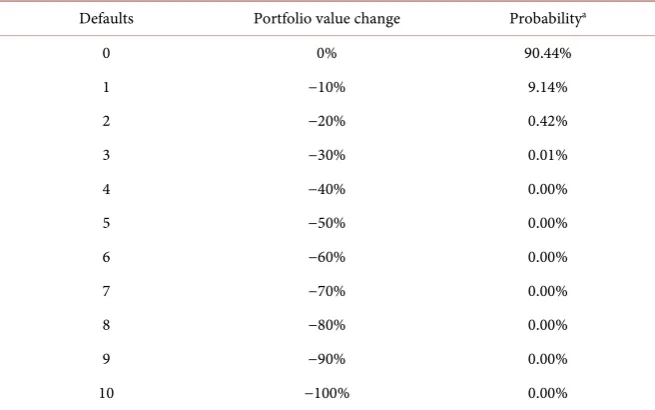
In the example of ten equally weighted issuers with an identical probability of default, the use of the binomial distribution yields the following results as illu-strated in Table 1.
The first two moments of the binomial distribution are defined as follows:
( )
E X =pτ (1)
( )
( )
1
E X
p
Var X p
n τ
τ −
= ∗ (2)
( )
X Va Xr( )
σ = (3)
where:
E expected value.
X default risk of the portfolio.
pτ default probability of an issuer over the period T. Var variance.
DOI: 10.4236/jfrm.2019.82007 95 Journal of Financial Risk Management Table 1. Binomial distribution, n = 10, p = 1%.
Defaults Portfolio value change Probabilitya
0 0% 90.44%
1 −10% 9.14%
2 −20% 0.42%
3 −30% 0.01%
4 −40% 0.00%
5 −50% 0.00%
6 −60% 0.00%
7 −70% 0.00%
8 −80% 0.00%
9 −90% 0.00%
10 −100% 0.00%
aBINOMDIST is a binomial distribution function. (Koshti, 2017: p. 8), (The Binomial Distribution, 2018:
pp. 2-11), (Habibi & Asgharzadeh, 2017: pp. 2-19) with the following parameters: 1) Number: Defaults; 2)
Trials: Total number of defaults; 3) Probability: 99%; 4) Cumulative: 0.
As can be seen from the above equations, the expected value of defaults is in-variant to the number of issuers, while the standard deviation decreases as the number of issuers increase.
For example, to calculate the issuer n—with the given variables:
standard deviation σ(X) = 1.41% and
default probability of an issuer over the period T pτ = 1%.
The second (2) equation and third (3) equation (as written above) need to be rearranged to achieve the variable n
(
)
( )
(
(
)
2)
1 1% 1 1%
50. 1.41%
p p
n
Var X
τ − τ ∗ −
= = =
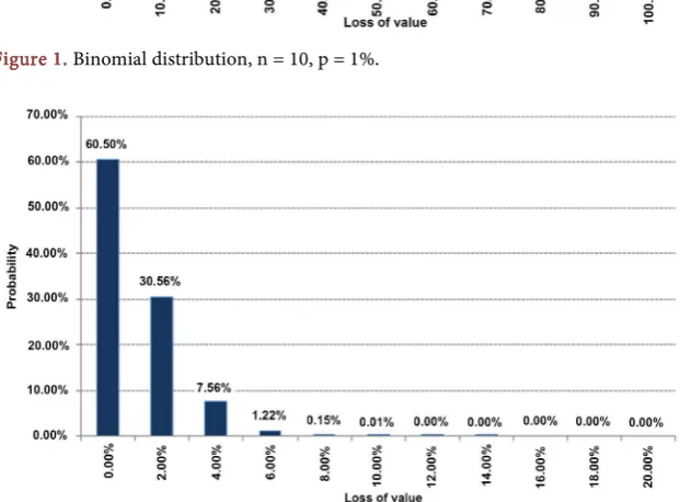
The consequences of a different standard deviation due to the different num-ber of issuers are shown in the following graphs, Figure 1 and Figure 2. They show the possible changes in the portfolio value due to the defaults in a portfolio of 10 issuers on the one hand and 50 issuers on the other hand.
The probability of losing 10% due to defaults is 9.14% for a portfolio of 10 is-suers is illustrated in Figure 1. The individual steps of the calculation are shown in Table 1.
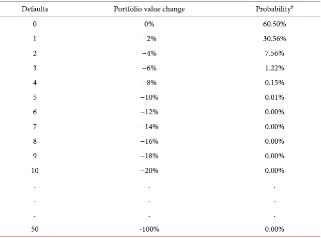
For a portfolio of 50 issuers to lose 10% requires five issuers to default.
The probability of this is only 0.01%. See Table 2 for an explanation of the Figure 2.
DOI: 10.4236/jfrm.2019.82007 96 Journal of Financial Risk Management Figure 1. Binomial distribution, n = 10, p = 1%.
Figure 2. Binomial distribution, n = 50, p = 1%.
However, the applicability of this methodology, as presented so far, is depen-dent on three main limiting assumptions:
1) the weights of the issuers are identical
2) the default probabilities of all issuers are identical 3) the defaults of issuers are independent on each other
Only in the rarest of cases these assumptions are applicable in practice. The rating agency Moody’s has developed a methodology called Binomial Ex-pansion Technique (BET) to abandon the restrictive assumptions of identical weights and default probabilities or uncorrelated default events and is still able to use binomial distribution in the valuation of CDOs. The complexity of the al-gorithm used by Moody’s makes it impractical to describe it in detail in the con-text of this paper and therefore a reference is made to the relevant literature4.
In essence, the approach can be summarized as follows:
4Moody’s Approach To Rating Synthetic CDOs BIS Working Papers No. 163, CDO rating
DOI: 10.4236/jfrm.2019.82007 97 Journal of Financial Risk Management Table 2. Binomial distribution, n = 50, p = 1%.
Defaults Portfolio value change Probabilityb
0 0% 60.50%
1 −2% 30.56%
2 −4% 7.56%
3 −6% 1.22%
4 −8% 0.15%
5 −10% 0.01%
6 −12% 0.00%
7 −14% 0.00%
8 −16% 0.00%
9 −18% 0.00%
10 −20% 0.00%
. . .
. . .
. . .
50 -100% 0.00%
bBINOMDIST is a binomial distribution function (Koshti, 2017: p. 8), (The Binomial Distribution, 2018:
pp. 2-11), (Habibi & Asgharzadeh, 2017: pp. 2-19) with the following parameters: 1) Number: Defaults; 2)
Trials: Total number of defaults; 3) Probability: 99%; 4) Cumulative: 0.
The objective of the approach is to calculate the expected loss of a portfolio and to assign a corresponding rating to that portfolio. As mentioned above, in order to apply the binomial distribution, Moody’s transforms an existing portfo-lio of issuers of different ratings, weights and dependencies into a synthetic portfolio that meets the conditions for applying the binomial distribution. The transformation of different default probabilities into a single one for the overall portfolio is not particularly difficult and can easily be accomplished by estab-lishing a weighted average5. In order to calculate the distribution of the expected losses, it is necessary to have—in addition to the probability of default—the in-put factor of the number of issuers or, in the terminology of the binomial distri-bution, the number of trials (n).
Moody’s algorithm makes it possible to calculate a synthetic number of issuers with the same weights from a portfolio with different weights of issuers of dif-ferent credit qualities. This value, which Moody’s calls the Alternative Diversity Score (ADS) (Fender & Kiff, 2004: pp. 4-5), may in some cases coincide with the actual number of issuers but generally differs from the actual number of issuers. The exact formula for ADS does not play a significant role in this paper, but is of great importance for the following line of reasoning (Fender & Kiff, 2004: pp. 4-5):
(
)
(
)
(
)
(
)
1 1
1 2 1 1
1
1 1
n n
i i i i
i i
n n
ij i i j j i j
i j
p F p F
ADS
p p p p F F
ρ
= =
= =
∗ −
=
− −
∑
∑
∑∑
DOI: 10.4236/jfrm.2019.82007 98 Journal of Financial Risk Management where:
Fi,j size of i and j position n number of positions
pi default probability of position i ρij pairwise default correlations
If it is assumed for a moment that the default probability of all issuers is iden-tical, then the formula is reduced to (Waibel, 2006: pp. 32-38):
1
1 2
1
i
n ij i j j
n
i n
i F ADS
Q F F =
=
=
=
∑
∑
∑
where:
Qij correlation matrix.
In this case, the ADS is completely independent of the default probability. Two portfolios with different probability of default will—ceteris paribus—have the same diversity score.
If the ADS is used as a measure of concentration, it would have the same value for a portfolio of 10 AAA issuers as for a portfolio of 10 BB issuers.
The basic idea of demanding a higher diversification from a portfolio with lower credit quality and correspondingly assigning a different degree of concen-tration is therefore not appropriate for the ADS. Its true purpose is solely as an input factor for the Moody’s binomial-based rating approach.
Both the HI and Moody’s ADS are of limited suitability in assigning a measure of diversification or concentration for the purpose of bond portfolios and mak-ing the portfolios directly comparable, takmak-ing into account both weights and de-fault probabilities of issuers.
An alternative to the existing concentration risk indicators is presented below.
3. Concentration Risk Indicator
This newly developed concentration ratio identifies potential concentration risks for positions that are not evenly built up in the portfolio. The measure is charac-terised by the fact that it focuses not only on the relative weights of issuers but also on their credit quality.
3.1. Initial Value
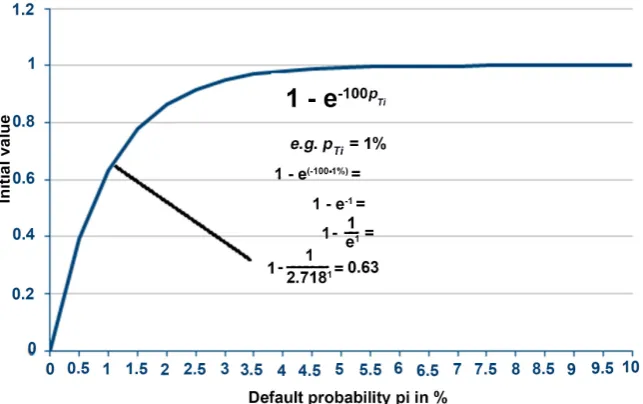
As a first step, it is to be assumed that a portfolio consists 100% of bonds issued by a single issuer. For an issuer with a very high credit quality (e.g. Germany or the USA) the concentration risk indicator is 0 due to the low probability of default, even when the issuer weight is 100%. As credit quality declines, the concentration indicator would increase exponentially when the issuer weight is 100%.
This relationship can be represented in an exponential function6 of the fol-lowing form, as illustrated in Figure 3:
6“exponential function f(x) = ex is the fact that the exponential function is the only nontrivial
DOI: 10.4236/jfrm.2019.82007 99 Journal of Financial Risk Management Figure 3. Single issuer portfolio and default probability piin %.
100
1 e− − pTi (4) pTi is the default probability of a rating category i for the period T.
In the case where the pTi is 0, the concentration indicator assumes a value of 0. As the default risk increases, the indicator approaches a value of 1.
A portfolio of, for example, 100% German government bonds would imply a concentration risk indicator of approximately 0, meaning the high credit quality of the issuer, Germany, would completely compensate for the 100% weight of the portfolio concentration.
3.2. Diversification Factor
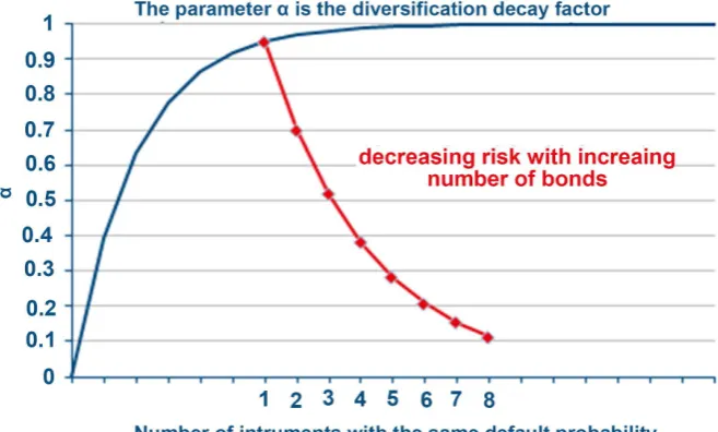
As a next step, a 1-issuer portfolio is no longer assumed and the concentration risk indicator is reduced by diversification. The concentration risk indicator thus decreases as the number of issuers increases, as shown in Figure 4.
The diversification factor (DF) is defined by the following equation:
1 1 100 i
i w
n
DF α
− − ∗
= (5)
where:
wi issuer weight of the portfolio, given that 0 ≤ wi ≤ 1.
ni required number of issuers, to be determined by risk preferences, e.g. the BB rating requires 100 issuers.
α diversification decay factor, given that 0 ≤ α ≤ ∞.
The value of α determines the “speed” of diversification, i.e. the gradient of the diversification curve, as illustrated in Figure 4.
DOI: 10.4236/jfrm.2019.82007 100 Journal of Financial Risk Management Figure 4. Reduction of the concentration risk indicator through diversification.
The exponent
1 1
100 i
i w
n
−
− ∗ expresses the ratio of actual weights and target
weights.
This calculation is carried out for each issuer and, as such, a concentration risk indicator value is generated for each individual issuer. The concentration risk indicator contribution for the overall portfolio is established by multiplying the concentration risk indicator value by the weights of the issuer, and the sum of these contributions gives the overall concentration risk indicator.
The concentration risk indicator (CRI) is thus defined as:
(
)
Weight Diversific1 1 1
ation Init
00* 100
ial Value 1 1 e
i
p iT i
w N
n i
i
CRI w α
− − −
=
=
∑
− ∗ ∗(6)
where:
N = number of issuers
α = diversification decay factor Ti
p = default probability of a rating category i for the period T i given that 0 < pTi ≤ 1
wi = % weight of an issuer i in a portfolio given that 0 < wi ≤ 1 ni = required number of issuers i dependent on the rating e = euler number with 2.7187
0 ≤ CRI ≤ 1 applies to the CRI where 0 means no concentration risk and 1 signals a high concentration risk.
CRI acknowledges the fact that low ratings generally require high diversifica-tion, e.g. an instrument with an AAA rating does not need to be diversified,
DOI: 10.4236/jfrm.2019.82007 101 Journal of Financial Risk Management whereas an instrument with a BB rating should be diversified. A portfolio with four BB-rated bonds has a lower CRI than a portfolio with three BB-rated bonds.
4. Practical Example
As a practical example, data from the bond portfolio described in Table 3 will be used to calculate a CRI ratio.
The steps involved in calculating the CRI ratio are enumerated below:
Step 1: As there are two identical issuers, the weights for the Polish issuers
will be added together, as specified in Table 4.
Step 2: A rating is assigned to each issuer.
Step 3: A probability of default p must be assigned to each rating as specified
by Moody’s credit rating.
Step 4: Determine the Initial Value as in Table 4.
Step 5: Determine the number of issuers ni as in Table 48.
Step 6: Determine the diversification factor DF, with α = 1.05 as in Table 4.
Step 7: Calculate CRI for each issuer as in Table 5.
Step 8: Add all the CRI values together to get the CRI ratio total for the
port-folio as in Table 5.
The CRI ratio for this example is 0.58. As mentioned, the CRI ranges from 0 to 1. Algorithm 1 shown below explains in detail the steps involved in calculating the CRI ratio:
Algorithm 1. Pseudocode for calculating CRI.
Result: CRI ratio for the portfolio Input: ISIN, Issuer, Rating, % Weight Output: CRI
Require: a minimum of one position in a portfolio 1) Aggregate the same issuers
if same issuer is repeated in portfolio then sum of weights for the same issuer end
2) Classify each rating
∀ issuer ∃ rating
3) Classify the default probability
∀ rating ∃ default probability pi, see Table 4
4) Calculate initial value
(
1 e− −100pTi)
, where pi is taken from step 3
5) Map the desired number of issuers
∀ rating ∃ ni
6) Calculate the diversification factor DF
1 1 100*
,
i i
w n
α
− −
given that α = 1.05
7) Calculate the CRI contribution per issuer Calculation: step 1 * step 4 * step 6 8) Aggregate the CRI ratio for each issuer
sum of all issuers from step 7
8n
i is freely selectable—better ratings result in a smaller number of required issuers and worse
DOI: 10.4236/jfrm.2019.82007 102 Journal of Financial Risk Management Table 3. Portfolio data example.
Type ISIN Issuer Rating % Weight
Bond TRT150120T16 Turkey BB+ 18.79
Bond HU0000402037 Hungary BBB− 9.45
Bond CZ0001002851 Czech A+ 15.63
Bond XS0638572973 Capital BB+ 10.00
Bond PL0000106670 Poland A− 20.85
Bond XS0767473852 Russia BB+ 5.35
Bond XS0800817073 VEB Fin. BB+ 4.32
Bond XS0841073793 Poland A− 7.96
Bond XS1028953989 Croatia BB 5.34
Bond XS1403619411 Krajo A− 2.31
[image:11.595.207.540.330.502.2]Source: Erste Asset Management database, May 2018.
Table 4. Constituents of the CRI calculation.
Issuer % Weight Rating p Initial Value ni DF
Turkey 18.79 BB+ 9.4 1.00 121 0.84
Hungary 9.45 BBB− 6.1 1.00 100 0.63
Czech 15.63 A+ 0.7 0.50 25 0.35
Capital 10.00 BB+ 9.4 1.00 121 0.70
Poland 28.81 A− 1.8 0.83 49 0.78
Russia 5.35 BB+ 9.4 1.00 121 0.49
VEB Fin. 4.32 BB+ 9.4 1.00 121 0.41
Croatia 5.34 BB 13.5 1.00 144 0.55
Krajo 2.31 A- 1.8 0.83 49 0.01
Table 5. CRI calculation for the portfolio.
Issuer CRI
Turkey 0.16
Hungary 0.06
Czech 0.03
Capital 0.07
Poland 0.19
Russia 0.03
VEB Fin. 0.02
Croatia 0.03
Krajo 0.00
[image:11.595.209.537.536.740.2]DOI: 10.4236/jfrm.2019.82007 103 Journal of Financial Risk Management
5. Summary
Various techniques for measuring, assessing and presenting concentration risks have been presented, and it has been determined that using existing scientific methods can produce misleading results.
In assessing concentration risks in bond portfolios, there is a two-dimensional problem insofar as the weight and credit quality of an issuer must be taken into account. For example, two portfolios that have the same number of issuers and equal weights but different issuer credit quality will have to be assessed diffe-rently in regards to their concentration risk.
This paper presents a credit risk adjusted diversification measure that is suita-ble for concentration risk assessment of bond portfolios using a single number, taking into account both weight and credit quality. CRI allows the identification of possible concentration risks within a large group of portfolios. Due to the standardised approach, CRI enables us to compare the concentration risk of dif-ferent portfolios.
Further research is required regarding the suitability of CRI for estimating the loss variance of a portfolio under stressed credit market conditions. The research thus far neither considered correlations between bonds in the portfolios, nor showed how it is expected to impact of portfolio return. Empirical evidence is therefore necessary concerning the input factor for loss estimation of CRI in comparison with approaches like the Herfindahl-Index and WARF and their corresponding ratios.
Conflicts of Interest
The authors declare no conflicts of interest regarding the publication of this pa-per.
References
Alsina, C., & Ger, R. (1998). On Some Inequalities and Stability Results Related to the Exponential Function. Journal of Inequalities and Applications, 2, 337-380.
https://doi.org/10.1155/S102558349800023X
http://www.kurims.kyoto-u.ac.jp/EMIS/journals/HOA/JIA/2/4373.pdf
Bank, St. Louis (2018). Simulation of the Hirfindahl-Hirschman Index: The Case of the St. Louis Banking Geographic Market.
http://www.siue.edu/GEOGRAPHY/ONLINE/zhou3.pdf
Fender, I., & Kiff, J. (2004). CDO Rating Methodology: Some Thoughts on Model Risk and Its Implications (p. 23). BIS Working Papers No. 163.
https://www.bis.org/publ/work163.pdf
https://doi.org/10.2139/ssrn.623662
Gioia, G. (2017). A Decomposition of the Herfindahl Index of Concentration.
https://mpra.ub.uni-muenchen.de/82944
Habibi, M., & Asgharzadeh, A. (2017). Power Binomial Exponential Distribution: Mod-eling, Simulation and Application. Communications in Statistics—Simulation and Com-putation, 47, 3042-3061. http://www.tandfonline.com/loi/lssp20
DOI: 10.4236/jfrm.2019.82007 104 Journal of Financial Risk Management In SPIE Smart Structures/NDE 2017 (pp. 1-28).
https://ntrs.nasa.gov/archive/nasa/casi.ntrs.nasa.gov/20170002582.pdf
Marling, H., & Emanuelsson, S. (2012). The Markowitz Portfolio Theory (pp. 1-6).
http://www.smallake.kr/wp-content/uploads/2016/04/HannesMarling_SaraEmanuelsso n_MPT.pdf
Mlbert, P. O. (2010). Corporate Governance of Banks after the Financial Crisis—Theory, Evidence, Reforms (pp. 1-45). ECGI—Law Working Paper.
https://papers.ssrn.com/sol3/papers.cfm?abstract_id=1448118
Moloney, N. (2010). Eu Financial Market Regulation after the Global Financial Crisis: “More Europe or More Risks”? Common Market Law Review, 47, 1317-1383.
http://www.kluwerlawonline.com/document.php?id=COLA2010058
Naldi, M., & Flamini, M. (2017). Censoring and Distortion in the Hirschman-Herfindahl Index Computation. Economic Papers: A Journal of Applied Economics and Policy, 36, 401-415. https://doi.org/10.1111/1759-3441.12187
https://www.researchgate.net/publication/319308320_Censoring_and_Distortion_in_t he_Hirschman-Herfindahl_Index_Computation
Naldi, M., & Naldi, M. (2014). The CR4 Index and the Interval Estimation of the Herfin-dahl-Hirschman Index: An Empirical Comparison. Hal Archives-Ouvertes.
https://hal.archives-ouvertes.fr/hal-01008144
https://doi.org/10.2139/ssrn.2448656
Qi, F., Niu, D.-W., & Guo, B.-N. (2017). Simplification of Coefficients in Differential Eq-uations Associated with Higher Order Frobenius-Euler Numbers.
https://www.preprints.org/manuscript/201708.0017/v1
https://doi.org/10.20944/preprints201708.0017.v1
Reynolds, D. (2009). Analyzing Concentration Risk. Algorithmics Software LLC.
https://pdfs.semanticscholar.org/0542/e1c0f2ef8ac298a1c22a36e18a31b4fd87d2.pdf Rhoades, S. A. (1993). The Herfindahl-Hirschman Index (pp. 188-189). St. Louis, MO:
Federal Reserve Bank of St. Louis.
https://fraser.stlouisfed.org/files/docs/publications/FRB/pages/1990-1994/33101_1990-1994.pdf
Semper, J. D. C., & Beltrn, J. M. T. (2011). Sector Concentration Risk: A Model for Esti-mating Capital Requirements. Mathematical and Computer Modelling, 54, 1765-1772.
https://www.sciencedirect.com/science/article/pii/S0895717710005789
https://doi.org/10.1016/j.mcm.2010.11.086
Tasche, D. (2006). Measuring Sectoral Diversification in an Asymptotic Multi-Factor Framework. Journal of Credit Risk, 2, 33-55. https://arxiv.org/abs/physics/0505142
https://doi.org/10.2139/ssrn.733084
The Binomial Distribution (2018). https://www3.nd.edu/~rwilliam/stats1/x13.pdf Tognetti, K. (1998). e the EXPONENTIAL—The Magic Number of GROWTH (pp. 1-32).
Wollongong: School of Mathematics and Applied Statistics, University of Wollongong.
https://www.austms.org.au/Modules/Exp/exp.pdf
Vo, L. H. (2015). Lessons from the 2008 Global Financial Crisis: Imprudent Risk Man-agement and Miss Calculated Regulation. Journal of Management Sciences, 2, 205-222.
https://www.researchgate.net/publication/297601761_Lessons_From_The_2008_Globa l_Financial_CrisisImprudent_Risk_Management_And_Miss_Calculated_Regulation
https://doi.org/10.20547/jms.2014.1502104
DOI: 10.4236/jfrm.2019.82007 105 Journal of Financial Risk Management Watt, R., & Quinto, J. (2003). Some Simple Graphical Interpretations of the Herfin-dahl-Hirshman Index and Their Implications (pp. 1-29). Working Document Univer-sidad Autnoma de Madrid and UniverUniver-sidad San Pablo CEU.
http://www.idee.ceu.es/Portals/0/Publicaciones/simple-graphical-interpretations-of-He rfindahl-Hirshman-Index.pdf
Yoshizawa, Y., & Witt, G. (2003). Moody’s Approach to Rating Synthetic CDOs (pp. 1-24). Moody’s Investors Service.