A robust and efficient adaptive multigrid solver for the optimal control of phase field formulations of geometric evolution laws

the optimal control of phase field formulations of

ge-ometric evolution laws

Feng Wei Yang1,∗_{, Chandrasekhar Venkataraman}2_{, Vanessa Styles}1_,

and Anotida Madzvamuse1

1_{Department of Mathematics, University of Sussex, UK}

2_{School of Mathematics & Statistics, University of St Andrews, UK}

Abstract. We propose and investigate a novel solution strategy to efficiently and ac-curately compute approximate solutions to semilinear optimal control problems, fo-cusing on the optimal control of phase field formulations of geometric evolution laws. The optimal control of geometric evolution laws arises in a number of applications in fields including material science, image processing, tumour growth and cell motil-ity. Despite this, many open problems remain in the analysis and approximation of such problems. In the current work we focus on a phase field formulation of the op-timal control problem, hence exploiting the well developed mathematical theory for the optimal control of semilinear parabolic partial differential equations. Approxima-tion of the resulting optimal control problem is computaApproxima-tionally challenging, requiring massive amounts of computational time and memory storage. The main focus of this work is to propose, derive, implement and test an efficient solution method for such problems. The solver for the discretised partial differential equations is based upon a geometric multigrid method incorporating advanced techniques to deal with the non-linearities in the problem and utilising adaptive mesh refinement. An in-house two-grid solution strategy for the forward and adjoint problems, that significantly reduces memory requirements and CPU time, is proposed and investigated computationally. Furthermore, parallelisation as well as an adaptive-step gradient update for the con-trol are employed to further improve efficiency. Along with a detailed description of our proposed solution method together with its implementation we present a number of computational results that demonstrate and evaluate our algorithms with respect to accuracy and efficiency. A highlight of the present work is simulation results on the optimal control of phase field formulations of geometric evolution laws in 3-D which would be computationally infeasible without the solution strategies proposed in the present work.

AMS subject classifications: 15A29, 35K58, 68W10

Key words: Optimal control, geometric evolution law, phase field, multigrid, parallel, mesh adap-tivity, two-grid solution strategy

∗_{Corresponding author.Email address:F.W.Yang@sussex.ac.uk(F.W. Yang)}

1

Introduction

The optimal control of geometric evolution equations or more generally free boundary problems arises in a number of applications. In image processing the tracking of de-formable objects may be formulated as the optimal control of a suitably chosen evolution law [1]. A number of applications arise from problems in material science such as the con-trol of nanosturcture through electric fields [2, 3]. An important and topical application area is the image driven modelling of biological processes, such as tumour growth [4] or cell migration [5], in which parameters (or functions) in a model are estimated from experimental imaging data. In a recent study we proposed an optimal control approach to whole cell tracking [6], i.e., the reconstruction of whole cell morphologies in time from a set of static images, in which the cell tracking problem was formulated as the optimal control of a geometric evolution equation [6]. In general the approximation of such op-timal control problems is computationally intensive both in terms of central processing unit (CPU) time and memory. Hence, the development of robust and efficient solvers for such problems with a view to reducing CPU time (or simply wall-clock time) and memory requirements is a worthwhile research direction.

In the current work we consider the optimal control of geometric evolution laws of forced mean curvature flow type. We denote byΓ(t), a closed oriented smoothly evolv-ingd−1 dimensional hypersurface in Rd_{,d=2,3 with outward pointing unit normalυυυ.} The motion ofΓ(t)satisfies a volume constrained mean curvature flow with forcing, i.e., given an initial surfaceΓ(0), the velocityVVVofΓ_{is given by}

VVV(xxx,t) = (−σH(xxx,t)+η(xxx,t)+λV(t))υυυ(xxx,t) xxx∈Γ(t),t∈(0,T], (1.1)

whereσ>_{0 represents the surface tension,Hdenotes the mean curvature (which we take} to be the sum of the principal curvatures) ofΓ_{,ηis a space time distributed forcing and} λV is a spatially uniform Lagrange multiplier enforcing volume constraint. We assume we are given an initial interfaceΓ0 _{and a target interface Γ}

obs both of which are smooth closed orientedd−1 dimensional hypersurfaces.

The optimal control problem, which is the focus of the current work, consists of find-ing a space time distributed forcfind-ingηin (1.1) such that withΓ(0) =Γ0_{, the interface}

be used (e.g., L2). In light of the above, we consider the phase field approximation of (1.1) given by the volume constrained Allen-Cahn equation, see (2.1). We approximate our initial and target data Γ0 _{and Γ}

obs by diffuse interface representations φ0 and φobs respectively (see for example [5] for details on how to construct such representations).

Our strategy for approximating the solution to the optimal control problem consists of an iterative adjoint based solution method, c.f., Sections 2 and 3. The method is partic-ularly computationally intensive for a number of reasons.

1. The iterative adjoint based solution method we employ necessitates multiple solves of the forward and adjoint problems.

2. As the state equation is of Allen-Cahn type grid adaptivity for the solution of the forward equation is mandatory for large simulations particularly in 3-D.

3. The computed state enters the adjoint equation which is posed backwards in time. Hence the state equation must first be solved over the whole time interval with the computed states stored and then the adjoint equation is solved backwards in time. Thus the algorithm requires large amounts of data storage.

4. We want to consider small values of the interfacial width parameter as many of the applications from cell biology that we are interested in involve interfaces with large curvatures and small scale features which we wish to resolve with our diffuse in-terface approximation. This imposes strong restrictions on the grid for the solution of the state problem.

In this work we focus on developing a robust and efficient solver for the problem. We employ a fast parallel adaptive multigrid solution method for the forward equation. The use of adaptive grids and parallelisation allows us to compute with relatively small val-ues of the interfacial width parameter. For the adjoint equation we make the observation that as the PDE is linear it may be possible to relax the restrictions on the grid needed for the solution of the state equation. Hence we employ a parallel multigrid solver for the adjoint equation on a uniform grid that is typically coarser than the adaptive grid used for the approximation of the state. We also consider a simple adaptive strategy for our iterative steepest descent based algorithm for the update of the control.

The remainder of this article is structured as follows. In Section 2 we present the opti-mal control problem and foropti-mally derive the optiopti-mality conditions used in the algorithm for its approximation. In Section 3 we describe our solver for the optimal control problem which is the main focus in this work. Firstly, in Section 3.1 we summarise the procedures required for solving this optimal control problem. We also outline the fully discrete meth-ods for the approximation of the state and adjoint equations in Section 3.2. We discuss the two-grid solution strategy in Section 3.3; and the adaptive-αalgorithm in Section 3.1 which improves the control update. Section 4 contains results of our numerical experi-ments with the implemented solver. We use a 2-D benchmark problem to demonstrate the convergence of the proposed model, our multigrid performance where a linear com-plexity is shown, effectiveness of the adaptive-α algorithm and two-grid strategy. We use a 3-D benchmark problem to illustrate the importance of the proposed two-grid solu-tion strategy in terms of the saved memory spaces. We also show 2-D and 3-D irregular shapes. Finally in Section 5 we summarise our major findings and discuss directions for future work.

2

Optimal control of a forced Allen-Cahn equation with volume

constraint

As outlined in Section 1 the prototype state equation we consider in this work consists of the volume constrained Allen-Cahn equation with forcing,

    

ǫ_∂∂_tφ(xxx,t) =ǫ△φ(xxx,t)−ǫ−1_G′_{(φ(xxx,t))+η(xxx,t)+λ(t) inΩ×(0,T],}

φ(xxx,0) =φ0(xxx) inΩ_,

∇φ(xxx,t)·υυυΩ(xxx) =0 on∂Ω,

(2.1)

whereφ(xxx,t)is the phase field variable, ǫ>_{0 is the parameter governing the interfacial} width of the diffuse interface, G(φ) =1

4(1−φ2)2 is a double well potential which has

minima at±1 and λis a time-dependent constraint on the mass that models a volume constraint [9] andυυυΩis the normal to∂Ω_.

As the volume enclosed by the target and initial interfaces may differ, i.e., R Ωφ06= R

Ωφobs, enforcing conservation of mass is inappropriate instead we proceed as in [6] and

enforce a constraint on the linear interpolation of the mass of the initial and target diffu-sive interfaces. To this end we define

Mφ(t):=

Z

Ω

φ0(xxx)+ t

T φobs(xxx)−φ 0_(xxx)

, (2.2)

and the volume constraintλ(t)in (2.1) is then determined such that fort∈(0,T]

Z

In order to formulate our optimal control problem we introduce the objective func-tional J, which we seek to minimise

J(φ,η) =1 2

Z

Ω(φ(xxx,T)−φobs(xxx))

2 dxxx+θ

2

Z T

0 Z

Ωη

2_{(xxx,t)dxxxdt, (2.4)}

whereθ>_{0 is a regularisation parameter. The first term of the right-hand side of (2.4) is} the so called fidelity term which measures the distance between the solution of the model and the target data φobs and the second term is the regularisation which is necessary to ensure a well-posed problem [8].

The optimal control problem we consider in this work may now be stated as the fol-lowing minimisation problem. Given initial data φ0 and target data φobs, find a space-time distributed forcingη∗:Ω×[0,T)→R_{such that withφa solution of (2.1) with initial} conditionφ(·,0) =φ0(·), the forcingη∗solves the minimisation problem

minηJ(φ,η), withJ given by (2.4). (2.5)

In order to apply the theory of optimal control of semilinear PDEs for the solution of the minimisation problem, we briefly outline the derivation of the optimality conditions, for further details see for example [8,10]. Adopting a Lagrangian approach, we introduce the Lagrange multiplier (adjoint state)pand the Lagrangian functionalL(φ,η,p)defined by

L(φ,η,p) =J(φ,η)−

Z T 0 Z Ω ǫ∂

∂tφ−ǫ△φ+ǫ

−1_G′_(φ)+η+λ

p. (2.6)

Assuming the existence of an optimal controlη∗ and the associated optimal stateφ∗

and requiring stationarity of the Lagrangian at(φ∗,η∗)yields the (formal) first order op-timality conditions [8, 10]

δφL(φ∗,η∗,p)φ=0, ∀φ:φ(xxx,t=0) =0, (2.7)

δηL(φ∗,η∗,p)η=0, ∀η. (2.8)

Condition (2.7) yields the linear parabolic adjoint equation posed backwards in time

     ∂

∂tp(xxx,t) =−△p(xxx,t)+ǫ−2G′′(φ(xxx,t))p(xxx,t) inΩ×[0,T),

p(xxx,T) =φ(xxx,T)−φobs(xxx) inΩ,

∇p(xxx,t)·υυυΩ(xxx) =0 on∂Ω×[0,T).

(2.9)

Condition (2.8) together with the Riesz representation theorem yields the optimality con-dition for the control [8]

δηL(φ∗,η∗,p) =θη∗+1

ǫp=0. (2.10)

3

Numerical solution methods

In this section, we outline the numerical methods for solving the proposed optimal con-trol of geometric evolution laws. For ease of exposition, we separate this complex solu-tion procedure into three parts. The first part, which deals with the update of the optimal controlη, is discussed in Section 3.1, with the assumption that the solutions ofφand p

have already been obtained. In Section 3.2, we describe the second part that involves the spatial and temporal discretization schemes for the forward (φ) and adjoint (p) problems, i.e., the phase field Allen-Cahn equation (2.1) with volume constraint and the adjoint equation (2.9) respectively. In order to solve this problem efficiently and accurately, we employ several state-of-the-art algorithms, described in Section 3.3, including an impor-tant in-house two-grid solution strategy, parallelised multigrid solution methods as well as dynamic adaptive mesh refinement. This forms the third and the last part of our solu-tion procedure.

3.1 Adaptive iterative update for the optimal control

The controlηis updated and obtained through an iterative approach, where the Allen-Cahn and adjoint equations (2.1) and (2.9) respectively, for each fixed time frame[0,T] have to be solved repeatedly. The computational requirement for finding a satisfactoryη

is large. This is mainly due to two reasons; first the necessity of repeatedly solving both Allen-Cahn and adjoint equations sequentially and second, the state (φ) and the forcing (η) must be stored at all iterations.

We denote a superscriptℓ_{for theηiteration, and at}ℓ_{=0, we take}

ηℓ=0=0 onΩ×[0,T) (3.1)

as our initial guess for the control. A better initial guess for the control may be necessary for certain examples or applications, however for the benchmark examples presented in this paper the simple constant zero initial guess stated above was sufficient for conver-gence.

For the purpose of demonstration, let us assume that both the state and adjoint equa-tions are solved by some known method with an acceptable accuracy. With this assump-tion, a gradient-based iterative update of the control, following the steepest descent ap-proach, is employed using (2.10) and the update is given by

ηℓ+1=ηℓ−α

θηℓ+1 ǫp

ℓ

, onΩ×[0,T), (3.2)

whereℓ_{+1 denotes the nextηiteration and}ℓ_{indicates the currentηiteration.}

and the latter takes the difference between the currentJand the previous one, and termi-nates when the difference between the two falls below a certain prescribed tolerance.

Due to the nature of the iterative update presented in (3.2), we expect each update on the controlηto reduce the objective functionalJ. Hence we design an adaptive algorithm based upon this observation. We may start with an arbitrary value ofα, namelyαℓ. If the computed objective function J withαℓ is smaller than the previous one, we increase the value of αℓ+1 and continue the computation. However, if J gets larger, this means the value αℓ is not suitable, and the computation with ηℓ need to be re-calculated using a smallerα(or the default minimum choiceαmin).

We summarise this adaptive procedure in Algorithm 1. NoteP_landPuare real num-bers, unless otherwise stated, we set them to be 0.5 and 1.1, respectively. In Section 4.4 we illustrate the effectiveness of this adaptive-αprocedure.

Algorithm 1Adaptive-α

1.While 1.While

1.While the difference between consecutive Js is still large or Jhas not reached below a pre-defined tolerance dododo

2. 2.

2. Solve the forward Allen-Cahn equation inΩ×(0,T] 3.

3.

3. Compute the objective functionalJℓ

4. 4. 4. ifififJℓ_>

Jℓ−1_{andandandℓ >0 thenthenthen}

α=max(α×Pl,αmin) restart = TRUETRUETRUE else if

else ifelse ifJℓ_<

Jℓ−1_{andandandℓ >0 thenthenthen}

α=α×Pu restart = FALSEFALSEFALSE end if

end ifend if 5. 5.

5. ififif restart == FALSEFALSEFALSE thenthenthen

Solve the backward adjoint equation inΩ×[T,0) Backup the currentη

Compute the nextηusingα

Continue to the nextηiteration else

elseelse

Compute a newηusing the latest backup withα

Restart the currentηiteration end if

end ifend if 6. End 6. End 6. End

3.2 Space-time discretizations of the forward Allen-Cahn and adjoint

equa-tions

a standard seven-point stencil in 3-D on Cartesian grids with cell-centred vertices. Al-though for illustrative purposes, the discrete system presented here is in 3-D, the use of a standard five-point stencil in 2-D is straightforward. We assumeNis the number of grid points in each coordinate direction,his the uniform grid spacing (i.e.h=△x=△y=△z), subscriptsi,j,kare used to indicate each grid point and each point has Cartesian coordi-nate(x,y,z). For the temporal discretization scheme we employ a fully-implicit second-order backward differentiation formula (BDF2) [11]. With a given end timeT, we assume a uniform time step sizeτ. For a time discrete sequence, f, we denote by fn:=f(tn). The standard BDF1 (also known as backward Euler method) is employed for the very first time step.

The result after applying the described discretisation to (2.1) is the following algebraic system arising at each time step, findφn+_i,j,k1,ℓ+1such that,

ǫφ

n+1,ℓ+1

i,j,k −43φ

n,ℓ+1

i,j,k +13φ

n−1,ℓ+1

i,j,k

τ =

2ǫ

3 D

φn+_i,j,k1,ℓ+1−

2

−φ_in+_,j,k1,ℓ+1+φ_in+_,j,k1,ℓ+13

3ǫ +

2η_in+_,j,k1,ℓ+1

3 +

2λn+1

3 ,

(3.3)

whereℓ_{+1 denotes the currentηiteration,n+1,nandn−1 indicate solutions from} cur-rent, previous and the one before the previous time steps, respectively. We denote the 3-D Laplacian operatorDas

D φi,j,k

=φi+1,j,k+φi−1,j,k+φi,j+1,k+φi,j−1,k+φi,j,k+1+φi,j,k−1−6φi,j,k

h2 . (3.4)

Within each time step, while solving for the solution of the above system, we are also required to satisfy a given mass constraint. This is done by iteratively determining the time-dependent, spatially-uniform volume constraintλ for the imposed mass con-straint [9]. Therefore, the system in (3.3) has to be solved multiple times, until a stopping criterion forλ is met. We denote thisλ iteration using a superscriptΛ_{, and its update} follows the multi-step approach presented in [9], which is given as

λn+1,Λ+1=λn+1,Λ+ λ

n+1,Λ_−λn+1,Λ−1h

M_φn+1−R Ωφn+1,

Λi R

Ωφn+1,Λ− R

Ωφn+1,Λ−1

, forΛ>1, (3.5)

whereMφis defined in (2.2),Λ+1,Λ_andΛ−1 indicate values ofλfrom current, previous and the one before the previousλiterations, respectively. We follow [9] in using the initial guesses

λΛ=0=−2ǫ τ +1,λ

Λ=1₌2ǫ

τ −1. (3.6)

The stopping criterion used here is based upon the difference between consecutive values of λ. Providing a tolerance tolλ, we consider the algorithm to have converged when

From our experience, using the initial guesses in (3.6) often led to more than threeλ

iterations within each time step (with, say, a typical choice oftolλ=0.01). For later com-putations, we can improve these initial guesses with known (already computed) values. Within the first and second η iterations, from time step n=3 onwards, we choose the computedλn−1,ℓandλn,ℓ, whereℓ_{=1,2, as our improved initial guesses. When we are at} the thirdηiteration or beyond, we choose the two computedλ(corresponding to the cur-rent time step) from the previous twoηiterations as initial guesses. It must be observed that the computed solutionφat each time step has to be stored in order to compute the adjoint stateplater.

Having solved the algebraic system arising from the discretizations of the phase field representation of (2.1) forward in time and stored the obtained solutions, we have only completed the first of two parts of the solution procedure. The second part is to discretize and solve (2.9). We employ the described central FDM and BDF2 as our discretization schemes, and the resulting algebraic system for the adjoint statepis the following,

pn+_i,j,k1,ℓ+1−4 3p

n+2,ℓ₊₁

i,j,k +13p

n+3,ℓ₊₁

i,j,k

τ =

−2

3D

pn+_i,j,k1,ℓ+1+2 3

  

−1+3φ_in+_,j,k1,ℓ+12

ǫ2 p

n+1,ℓ+1

i,j,k

  .

(3.7)

Note that the adjoint equation is posed backwards in time and its terminal condition is stated in (2.9). The BDF1 method needs to be employed for the first time step. For every subsequent time step the corresponding solution ofφthat has been previously computed and stored enters as data in the adjoint equation.

3.3 Techniques for improving algorithm efficiency

We propose a two-grid solution strategy that exploits a key difference between the forward Cahn and the backward adjoint equations. As is well known for the Allen-Cahn equation the parameterǫdetermines the thickness of the diffuse interfacial region, Γ_ǫ, that approximates the hypersurfaceΓ. In order for the Allen-Cahn equation to reliably approximate mean curvature flow the interfacial region has to be well resolved. Typically eight grid points are required across the width of the diffusive interface, see [16]. On the other hand, in our numerical simulations we observed that the solution of the backward adjoint equation varies less, see Figures 4 (c) and 4 (d) in which the optimised solutions of the adjoint equation at time t=0.0625 and t=0.125 are displayed, and so a milder restriction on the grid sizehin the interfacial region is expected when solving this equa-tion. Our numerical tests (see Section 4) suggest that such a strategy can dramatically reduce the memory requirement and increase computational efficiency without signifi-cantly compromising accuracy.

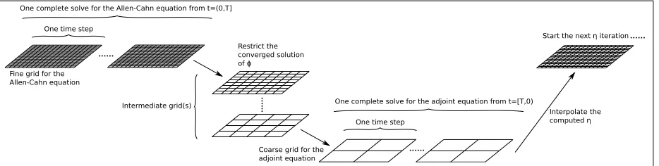
Within this implemented robust in-house two-grid solution strategy, we solve the Allen-Cahn equation on a grid hierarchy where its finest grid has sufficient grid points for the chosenǫ; the backward adjoint equation is then solved using only part of the grid hierarchy to improve the efficiency. As we stated previously, during the computation, at least solutions from two variables ofφ, pandηfrom all time steps in the currentη iter-ation are stored. If a very fine mesh resolution is required, this undoubtedly imposes a severe requirement for the memory, even in a parallel setting. To relax this constraint, we store all-time-step solutions only on the coarser grid where we solve the adjoint problem. When the stored solutions are required on finer grids (whereφis solved), an interpola-tion is used to transfer the stored soluinterpola-tions to that grid level. We illustrate this two-grid solution strategy in Figure 1.

One time step

One complete solve for the Allen-Cahn equation from t=(0,T]

Intermediate grid(s)

Restrict the converged solution of

Fine grid for the Allen-Cahn equation

Coarse grid for the adjoint equation

One time step

One complete solve for the adjoint equation from t=[T,0)

Interpolate the computed Start the next iteration

Figure 1: Sketch illustrating our in-house two-grid solution strategy, where the adjoint equation is solved on a much coarser grid. The storage for all-time-step solutions is done on such a grid so as to reduce the memory requirement.

Remark 3.1. When solving such optimal control problems we note that apart from the

every grid point at every time step. For the adjoint equation (2.9), the solution of the state equationφon every space-time grid point is also required. Thus, when we solve the Allen-Cahn equation, the solutions of φandηare stored on every grid point for all time steps. The requirements on memory storage can become significant as the number of grid point increases.

To give the reader a brief idea, say one uses a 2-D grid consisting of 5122 grid points with 50 forward and backward time steps for the Allen-Cahn and the adjoint equation respectively. The solutions of 2 variables (φandη) are stored using a double-precision format, i.e., each float-point number occupies 8 bytes in the memory. This setting requires around 210 megabytes of memory space. However, if this simulation is done in 3-D on a uniform grid with the resolution of 5123_{, the memory requirement becomes}

approxi-mately 107 gigabytes. Such a simulation may not be feasible if no parallelism nor any other advanced techniques are employed. To this end, we couple our two-grid solution strategy with a parallelisation of a domain decomposition approach, as well as dynamic AMR to enable 3-D simulations.

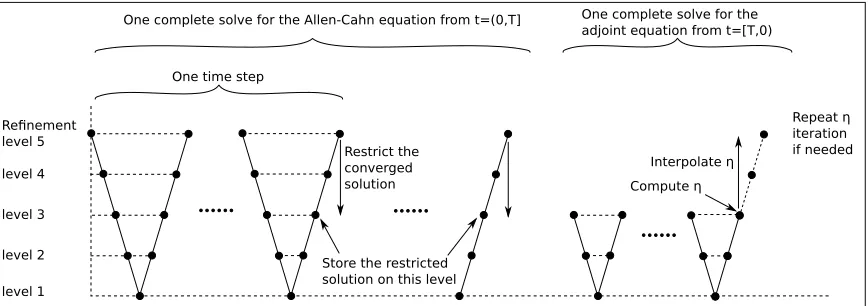
The software framework used here is called Campfire v2.0. Comparing with its pre-vious versions used in [12–14], the latest software received some significant changes to its structure in order to deal with a forward and a backward solve, as well as additional parallel memory allocations. This framework contains a geometric nonlinear multigrid solution method with a full approximation scheme (FAS), as well as a multi-level adap-tive technique (MLAT) variant. However, when solving the linear adjoint equation, this FAS multigrid reduces to the standard linear multigrid method [17]. The multigrid meth-ods are widely known to be one of the fastest numerical methmeth-ods with a linear complex-ity [17–19], and we later demonstrate this in the paper. Its parallelisation comes from a domain decomposition technique, and message passing interface is used for parallel communication. Here using Figure 2, we illustrate that the presented in-house two-grid solution strategy can be comfortably extended into the multigrid V-cycles.

level 1 level 2 level 3 level 4 Re nement level 5

One time step

One complete solve for the Allen-Cahn equation from t=(0,T]

Restrict the converged solution

Store the restricted solution on this level

One complete solve for the adjoint equation from t=[T,0)

Compute Interpolate

Repeat iteration if needed

Figure 2: Sketch demonstrating our in-house multi-depth V-cycle multigrid strategy where the adjoint equation is solved on a much coarser grid. The storage for all-time-step solutions is done on such a grid so as to reduce the memory requirement.

4

Numerical experiments

All the results shown in this section were generated using the local HPC cluster provided and managed by the University of Sussex. This HPC cluster consists of 3000 computa-tional units. The models of the computacomputa-tional units are AMD64, x86 64 or 64 bit archi-tecture, made up of a mixture of Intel and AMD nodes varying from 8 cores up to 64 cores per node. Each unit is associated with 2GB memory space. Most of the simulations in this paper were executed using 4−32 cores. The parallel scalability of our multigrid solver, Campfire, has been discussed in earlier publications such as [12–14], where in [12], they successfully scaled up to one thousand computational cores on the national super-computer VECToR in 2013. We refer the reader to [13, 14] for a detailed explanation and related results for the parallel scalability of our software.

4.1 A 2-D benchmark example

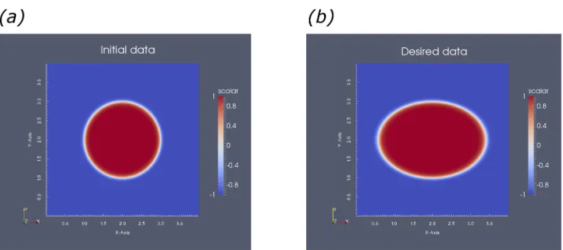
We start with a benchmark 2-D example. The initial data is a circle centred at(2,2)with radius 1. We use a hyperbolic tangent function to obtain a continuous interfacial region with a width ofO(ǫ)

φt=0=tanh

 

−h(x−2)2+(y−2)2−1

i

ǫ



. (4.1)

The desired data is an ellipse:

φobs=tanh

  

−h(x−₂2)2+(y−2)2−1i

ǫ

 

Both the initial and desired shapes are illustrated in Figure 3.

For illustrative purposes, we take the computational domainΩ= (0,4)2_{. The choices}

of parameters are given in Table 1. At each time step, the infinity norm of the residual is assessed, and the computation is said to be converged when this norm is smaller than 1.0×10−11_.

Name Description Value

α Step size for the control update 0.1

θ Regularisation parameter 0.01

ǫ Width of the diffuse interface 0.1

T Total time duration 0.125

τ Time step size (varies)

Table 1: The parameters of the optimal control problem for the 2-D examples.

Figure 3: (a) shows the initial data (i.e. (4.1)) and (b) shows the desired data (i.e. (4.2)). The colour version of this figure is online.

We present the computed solutions from a uniform grid with a resolution of 10242_.

We select a time stepτ=7.8125×10−4, which yields 160 time steps. For the propose of demonstration, we run 50ηiterations. In a multigrid setting, we use a 162as the coars-est grid, and grids like 322, 642 etc. are the intermediate grids in the V-cycle hierarchy. The multigrid hierarchy is used for all simulations (163used as the coarsest grid for 3-D simulations) and is fairly standard, for clarity we forgo mentioning the multigrid setting later on.

included in Figures 4 (c) and (d). The corresponding solutions ofηare shown in Figures 4 (e) and (f). We can see that, as expected for a circle evolving into an ellipse, the most forcing in (c) is placed at the left and the right. We also observe that in (d), the forcing is highly positive on the inner side of the phase field interface, and highly negative on the other, in order to keep the shape from further unwanted expansion or shrinking. The reductions in the objective functionalJ from the 50ηiterations are shown using a semi-log plot in Figure 7 as “fixed alpha”.

4.2 Convergence tests for the benchmark 2-D example

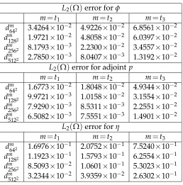
L2(Ω)error forφ

m=t1 m=t2 m=t3 d₆₄m2 3.4264×10−2 4.9226×10−2 6.8561×10−2 d₁₂₈m 2 1.9721×10−2 4.8058×10−2 6.0397×10−2 d₂₅₆m 2 8.1793×10−3 2.2300×10−2 3.4557×10−2 dm

5122 2.7850×10−3 8.0407×10−3 1.3192×10−2 L2(Ω)error for adjoint p

m=t1 m=t2 m=t3 d₆₄m2 1.6773×10−2 1.8048×10−2 4.9344×10−2 dm

1282 9.9721×10−3 1.0158×10−2 3.1554×10−2 dm

2562 7.9290×10−3 8.5311×10−3 2.2551×10−2 d₅₁₂m 2 6.5082×10−3 7.5551×10−3 1.4901×10−2

L2(Ω)error forη

m=t1 m=t2 m=t3 dm

642 1.6976×10−1 2.0752×10−1 7.5240×10−1 dm

1282 1.1923×10−1 1.5793×10−1 6.2554×10−1 d₂₅₆m 2 8.5093×10−2 1.0601×10−1 5.3023×10−1 d₅₁₂m 2 3.2344×10−2 3.9359×10−2 2.6302×10−1

Table 2: The convergence tests for the solutions ofφ, adjoint pandη.

In this subsection, we report on numerical evidence that the proposed optimal control model converges as we refine both spatially and temporally.

We use the simulation that was described in the previous subsection as a benchmark. To recap, it was solved on a grid with the resolution of 10242 and 160 number of time steps.

In order to conduct the convergence tests, the optimal control model here is solved independently on the following grids: 642, 1282, 2562and 5122. We use a time step size

τ=0.0125 for the 642_{simulation, which has 10 time steps. Then the choices ofτis halved}

(a) (b)

(c) (d)

(e) (f)

shown in Table 1. However, instead of running theηiteration to a constant, we change the stopping criterion so that theηiteration stops when the objective functionalJis below 0.065. Note this new stopping criterion requires 24ηiterations to be satisfied for the 10242 simulation and roughly the same for other simulations.

We assess the solutions generated at three specific times. They are t1=0.0125, t2=

T/2=0.0625 andt3=T=0.125. Notet1is at the end of first time step of the 642_simulation,

and subsequently the end of second, fourth and eighth time steps of the 1282, 2562 and 5122simulations respectively.

To compare the solutions spatially at the correspondingt1, t2 andt3, further proce-dures are required. This is because the solutions are generated with different resolutions of grids. As mentioned earlier, we use the solution from 10242 _{grid as the benchmark,}

therefore all the solutions from other simulations other than 10242are interpolated to the uniform 10242 grid. Note this process uses a standard bilinear interpolation [17], which is also the one used in our multigrid solver.

The interpolated solutions are compared with the benchmark solutions att1,t2andt3. Solutions from all grid points are assessed for the difference from the benchmark solution in theL2(Ω)error defined as follows

dm_l :=∑ N

i=1∑Nj=1(φim,j,l−φm,1024

2

i,j )2

N×N , m=t1,t2,t3, l=64

2_,1282_,2562_,5122 _(4.3)

whereφ_im_,j,l is the computed and interpolated value ofφ on grid l and N=1024 is the number of internal grid points (after interpolation) on one axis. This is repeated for the solutions of the adjointpandη. We summarise the convergence tests in Table 2. It can be seen from this table that as we refine both spatially and temporally, the solutions of the proposed optimal control model appear to converge.

4.3 The multigrid performance on the benchmark 2-D example

Within our software framework, the algebraic system arising from each time step is solved by a multigrid solver. Here in this subsection, we assess, numerically, the per-formance of our multigrid perper-formance.

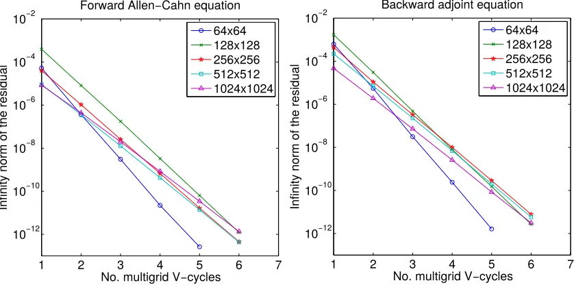
First of all, we present multigrid convergence rates by plotting the infinity norm of the residual at the end of each V-cycle from a typical time step. Furthermore, since two different equations are solved separately, we separate them and illustrate these results in Figure 5. All eight lines from two plots in Figure 5 are nearly parallel to each other which suggests the reductions in the infinity norms of the residuals are independent of grid sizes.

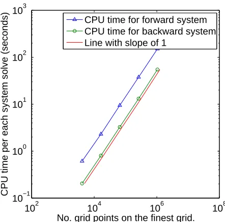
We demonstrate the linear complexity of our multigrid solver in Figure 6. Five sim-ulations (642_{, 128}2_{, 256}2_{, 512}2_{and 1024}2_{) are timed with a single computational core and}

1 2 3 4 5 6 7 10−12

10−10

10−8

10−6

10−4

10−2

No. multigrid V−cycles

Infinity norm of the residual

Forward Allen−Cahn equation

64x64 128x128 256x256 512x512 1024x1024

1 2 3 4 5 6 7

10−12

10−10

10−8

10−6

10−4

10−2

No. multigrid V−cycles

Infinity norm of the residual

Backward adjoint equation

64x64 128x128 256x256 512x512 1024x1024

Figure 5: The multigrid convergence rates for the forward Allen-Cahn and backward adjoint equations. The colour version of this figure is online.

because, the volume constraint typically requires 2 - 3 choices ofλ(more in the first two

ηiterations, since the guesses forλare poor), meaning the algebraic system from the for-ward equation has to be solved 2 - 3 times within each time step. On the other hand, the algebraic system for the backward equation only requires to be solved once.

4.4 Adaptive-αalgorithm with the benchmark 2-D example

An additional improvement to the efficiency may come from using the described

adaptive-αalgorithm (see Algorithm 1). In this subsection, we illustrate the effectiveness of this approach.

The two most influential parameters in the algorithm arePlandPuwhich control the incremental and decremental portions of the step size respectively. For the purpose of demonstration, we use the described 10242simulation with 160 time steps. As mentioned previously, the reductions of the objective functional J within a fixed 50η iterations is shown in Figure 7 (a). The initial choice of αℓ=0=0.1 is the same used in the fixed α

simulations previously.

Here we choose three different incremental parameters: P1

u=110%, Pu2=120% and

P3

u=130%. The corresponding decremental parameters are Pl1=50%, Pl2=40% and

P3

l =30%, respectively. Thus the more increases to the step size, the harder the penal-isations become. For comparison, simulations with these three pairs of parameters are done with 50 fixedηiterations. We plot the reductions of the objective functionalJ from using the adaptive-αalgorithm in Figure 7 (a). Note that in this figure, we only show the

102 104 106 108 10−1

100 101 102 103

No. grid points on the finest grid.

CPU time per each system solve (seconds)

CPU time for forward system CPU time for backward system Line with slope of 1

Figure 6: A log-log plot to illustrate the linear complexity of our multigrid solver. For comparisons, a line of slop1is included. The colour version of this figure is online.

all four simulations in Figure 7 (b), where the decreases in the values ofαindicate the failed attempts. A trade-off can be observed from these two figures: a larger incremental parameter leads to a faster convergence, however, this may result in more failed attempts and thus in turn results in more computational time. In this case the gains in efficiency of the adaptive-αapproach against a fixed value ofαare evident. The use of an adaptive

αis motivated by the fact that in general our initial guess for the solution to the optimal control problem may be poor and hence large step sizes may be admissible in the steep-est descent update as we are far from local minima. As we approach the local minima smaller step sizes are necessary to prevent overshoot and hence some adaptivity in the parameterαis expected to be desirable. More involved algorithms for the selection of an optimal parameterα, e.g., via a line search [8], may also be worthwhile topics of future investigation.

4.5 Two-grid solution strategy with dynamic AMR on the benchmark 2-D

ex-ample

(a) _(b)

Figure 7: A semi-log plot shows the reductions of the objective functional J from using constant and adaptive

αs in (a). A semi-log plot shows the changes in the values ofαin (b). The colour version of this figure is online.

dynamic AMR.

We consider a two-grid simulation where we solve the forward Allen-Cahn equation on a 10242 _{uniform grid while the adjoint equation and the storage of all the solutions,}

η, φ, p, takes place on a 642uniform grid. The solutions of this two-grid simulation are compared with solutions using a standard (one-grid) 642 uniform grid simulation. We note that in both simulations all solutions are stored on a grid with resolution of 642_.

For simplicity, we take 160 time steps for both simulations so that temporal errors have less influence. Like the convergence tests shown in Subsection 4.2, we solve the system until J gets below 0.065. In order to compute the error, the solutions from both simulations are interpolated and compared against solutions from the 10242simulation.

We illustrate the errors in Table 3, where

dm₁₀₂₄2₋₆₄2:=

∑N_i=1∑N_j=1(φm_i,j,10242−642−φm_i,j,10242)2

N×N , m=t1,t2,t3,

withφ_im_,j,10242−642 denoting theφsolution from the two-grid simulation.

From this table we see that solving φon a finer grid, while solving for pon a coarse grid and storing all solutions on the coarse grid, not only results in a reduction of the error inφbut it also results in a reduction of the errors ofpandη. However since the number of degrees of freedom in the two-grid (10242₋₆₄2_{) simulation is considerably larger than}

the number of degrees of freedom in the standard 642 simulation. This behaviour is somewhat expected. In the next simulation we conduct a comparison between a two-grid simulation that solves the Allen-Cahn equation on an adaptive 2562 _{grid with dynamic}

L2(Ω)error forφ

m=t1 m=t2 m=t3 d₆₄m2 3.1224×10−2 4.7216×10−2 6.3531×10−2 dm₁₀₂₄2₋₆₄2 8.1840×10−3 1.6194×10−2 8.6616×10−3

L2(Ω)error for adjoint p

m=t1 m=t2 m=t3 d₆₄m2 1.3722×10−2 1.2018×10−2 4.0874×10−2 dm₁₀₂₄2₋₆₄2 6.1444×10−3 4.9266×10−3 9.9998×10−3

L2(Ω)error forη

m=t1 m=t2 m=t3 d₆₄m2 1.2176×10−1 1.8872×10−1 6.9943×10−1 dm₁₀₂₄2₋₆₄2 9.9110×10−2 1.3768×10−1 4.2063×10−1

Table 3: Comparisons of errors between a two-grid simulation (10242₋₆₄2_{) and a standard64}2 _simulation.

simulations is comparable, 17200 (maximum number of degrees of freedom occurred) for the two-grid simulation versus 1282=16384.

Both simulations have 160 time steps. The errors are shown in Table 4. From this table, we can see that for the two-grid simulation only the errors inφare better. This is expected as the adjoint is solved on a coarser grid (i.e. 642_{) andη,φandpare stored on this coarse}

grid. On the other hand, it is important to note that we can store all the solutions on a coarser grid as well as solving the adjoint equation there without compromising too much on accuracy; this is crucial for 3-D simulations. In Figure 8 we show two snapshots of our dynamic AMR att=t1andt=T.

4.6 3-D example

We mentioned previously in Remark 3.1 that solving a 5123_{3-D simulation using a}

stan-dard uniform grid requires memory of over 100 gigabytes space. Using the two-grid solution strategy and dynamic AMR for the phase field variable, we can run a 5123 sim-ulation with less than 20 gigabytes memory requirement. This simsim-ulation is done in a 3-D domainΩ= (0,1)3_{. We choose a uniform 64}3 _{to be the grid where we store all the}

solutions and solve the adjoint equation. The finest grid is an adaptive grid and if it was to become uniform, it would have the resolution of 5123_{. The temporal domain is}

L2(Ω)error forφ

m=t1 m=t2 m=t3 dm₁₂₈2 1.2327×10−2 2.6664×10−2 3.8450×10−2 d₂₅₆m 2₋₆₄2 8.6270×10−3 1.6895×10−2 3.2925×10−2

L2(Ω)error for adjointp

m=t1 m=t2 m=t3 dm₁₂₈2 9.2021×10−3 9.7122×10−3 3.0233×10−2 d₂₅₆m 2₋₆₄2 1.0004×10−2 1.4886×10−2 2.7392×10−2

L2(Ω)error forη

m=t1 m=t2 m=t3 dm₁₂₈2 9.7196×10−2 1.2153×10−1 5.3632×10−1 d₂₅₆m 2₋₆₄2 7.7932×10−2 1.4930×10−2 5.9167×10−1

Table 4: Comparisons of errors between an adaptive two-grid simulation (2562₋₆₄2_{) with AMR and a standard} 1282 _{uniform grid simulation.}

0 1 2 3 4

0 0.5 1 1.5 2 2.5 3 3.5 4

AMR at t1 (first time step)

Domain in x axis

Domain in y axis

0 1 2 3 4

0 0.5 1 1.5 2 2.5 3 3.5 4

AMR at t=T (end time)

Domain in x axis

Domain in y axis

Figure 8: Two colour plots show the dynamic AMR in our solver. The blue region shows the 644 _{grid; light} green region indicates the1282 grid; and finally red region illustrates the finest2562 grid. The colour version of this figure is online.

We define the initial shape to be a sphere

φt=0=tanh

 

−h(x−0.5)2+(y−0.5)2+(z−0.5)2−0.252i

ǫ



and the desired data to be an ellipsoid

φobs=tanh

  

−h(x−₂0.5)2+(y−0.5)2+(z−0.5)2−0.252i

ǫ

 

. (4.5)

The zero-isosurface ofφfor both the initial and desired shapes are illustrated in Figure 9 (a) and (b) respectively. Following a fixed 15η iterations, we present two plots of the zero-isosurface ofφ in Figure 9 (c) and (d). The solution in (c) is halfway through the temporal domain and the solution in (d) is the computed final shape. We use colours and colour-value indicator on the side to demonstrate the corresponding solutions ofηon the zero-isosurface. The reductions of the objective functionJ are shown in Figure 10.

4.7 Irregular shapes

In all our previous simulations we used relatively simple shapes for illustrative purposes only. In this subsection, we show some irregular shapes in both 2-D and 3-D in order to illustrate that the proposed optimal control approach is capable of dealing with general interfaces.

We start with a 2-D example which takes a circle as the initial shape and the desired shape is the following

φobs=max

(

tanh

  

−h[(x−2)+(y₆ −2)]2+[(y−2)−₁(x−2)]2−1i

ǫ   , tanh   

−h[(x−2)+(y₆ −2)]2+[(y−2)−₁(x−2)]2−1i

ǫ    ) . (4.6)

We take the computational domainΩ= (0,4)2_{and use the parameters presented in Table}

1. This simulation is solved using a two-grid approach which has a 5122 grid for the Allen-Cahn and a 642 for the adjoint equation. We setT=0.05 and use a time step size

τ=0.001. The initial and desired data are illustrated in Figure 11. We present our results in Figure 12, which include the solutions ofφat the first time step, the halfway mark (i.e.

t=0.0025) and the end time, together with their corresponding controlη. We define two 3-D shapes as follows

φ0=tanh

    −

2(x−2)−(z−2)22+(y−2)2+(z−2)2−1

ǫ

  

(a)

(b)

(c)

(d)

Figure 10: A semi-log plot shows the reductions of the objective functionJ. The colour version of this figure is online.

φobs=tanh

   

−

(y−2.3)−(z−2.3)22+2(x−2.3)2+(z−2.3)2−1

ǫ

   

. (4.8)

The simulation has the same setting as the one described in Subsection 4.6 and we illustrate the zero-isosurface together with the values of the optimal control η on this isosurface in Figure 13.

(a)

(b)

(c)

_(d)

Figure 13: Figures (a) and (b) show the zero-isosurface ofφof initial data and desired data respectively; (c) and (d) illustrate the zero-isosurface of computed solutions halfway through (i.e. t=T/2) and the final shape (i.e.

5

Conclusion

In this work, we focussed on the development of robust and efficient solution procedures for the approximation of the optimal control of geometric evolution laws using phase field formulations, the problems under consideration arise naturally in many applica-tions [1–3, 8, 10]. Such optimal control problems are very computationally-demanding and memory hungry especially when posed in three dimensions. Thus the development of an efficient, robust and accurate solver is of much importance. We have described, in detail, a solution procedure that combines a number of state-of-the-art algorithms to im-prove overall efficiency. We employed a steepest descent approach for the iterative com-putation of the optimal control. We introduced an adaptive-step-size algorithm which tries to use as large a step size as possible to reduce the number of iterations needed. Robust and efficient solvers for both the forward (Allen-Cahn) and adjoint equations, based on FAS multigrid methods with MLAT are described together with their parallel implementation which is crucial for minimising wall clock time due to the massive mem-ory requirements. We discussed the use of mesh refinement which dramatically reduces the number of degrees of freedom required for the solution of the forward problem, and is crucial in terms of reducing the computational complexity. A major finding of this work is that a two-grid solution strategy, in which the forward equation is solved on an adaptively refined grid whilst the adjoint problem is solved on a coarser grid, thus signif-icantly reducing CPU and memory requirements, appears to lead to only a minor loss in accuracy. We have implemented our algorithms and conducted detailed tests and bench-marks of our solution methods using 2-D and 3-D examples. The conclusion is that our solution algorithms can significantly improve efficiency while maintaining an acceptable accuracy.

Data Management

All the computational data output is included in the present manuscript.

Acknowledgements

All authors acknowledge support from the Leverhulme Trust Research Project Grant (RPG-2014-149). The work of CV, VS and AM was partially supported by the Engineering and Physical Sciences Research Council, UK grant (EP/J016780/1). This work (AM) has also received funding from the European Union’s Horizon 2020 research and innovation programme under the Marie Sklodowska-Curie grant agreement No 642866. The work of CV is partially supported by an EPSRC Impact Accelerator Account award. The au-thors (FWY, CV, VS, AM) thank the Isaac Newton Institute for Mathematical Sciences for its hospitality during the programme (Coupling Geometric PDEs with Physics for Cell Morphology, Motility and Pattern Formation; EPSRC EP/K032208/1). AM was partially supported by Fellowships from the Simons Foundation.

References

[1] Papadakis, N. and M´emin, E., Variational optimal control technique for the tracking of de-formable objects, Computer Vision, IEEE 11th International Conference, 1-7, 2007.

[2] Haußer, F., Rasche, S. and Voigt, A., The influence of electric fields on nanostructures-simulation and control, Mathematics and Computers in Simulation, 80(7), 1449-1457, 2010. [3] Haußer, F., Rasche, S. and Voigt, A., Control of nanostructures through electric fields and

re-lated free boundary problems, in: Constrained Optimization and Optimal Control for Partial Differential Equations, 561-572, 2012.

[4] Hogea, C., Davatzikos, C. and Biros, G., An image-driven parameter estimation problem for a reaction–diffusion glioma growth model with mass effects, Journal of mathematical biology, 56(6), 793-825, 2008

[5] Croft, W., Elliott, C.M., Ladds, G., Stinner, B., Venkataraman, C. and Weston, C., Parameter identification problems in the modelling of cell motility, Journal of Mathematical Biology, 71(2), 399-436, 2015.

[6] Blazakis, K.N., Madzvamuse, A., Reyes-Aldasoro, C.C., Styles, V. and Venkataraman, C., Whole cell tracking through the optimal control of geometric evolution laws, Journal of Computational Physics, 297, 495-514, 2015.

[7] Vierling, M., Parabolic optimal control problems on evolving surfaces subject to point-wise box constraints on the control–theory and numerical realization, Interfaces and Free Bound-aries, 16(2), 137-173, 2014.

[8] Tr ¨oltzsch, F., Optimal control of partial differential equations: theory, methods and applica-tions, AMS Bookstore, 112, 2010.

[9] Blowey J. and Elliott C., Curvature dependent phase boundary motion and parabolic double obstacle problems, In Degenerate Diffusions, 51, 52, 55, 19-60, 1993.

[11] Emmerich, E., Stability and error of the variable two-step BDF for semilinear parabolic prob-lems, Journal of Applied Mathematics and Computing, 19, 33-55, 2005.

[12] Bollada, P., Goodyer, C., Jimack, P., Mullis, A. and Yang, F., Thermalsolute phase field three dimensional simulation of binary alloy solidification, Journal of Computational Physics, 287, 130-150, 2015.

[13] Yang, F.W., Goodyer, C.E., Hubbard, M.E. and Jimack, P.K., Parallel implementation of an adaptive, multigrid solver for the implicit solution of nonlinear parabolic systems, with ap-plication to a multi-phase-field of tumour growth, Proceedings of the Fourth International Conference on Parallel, Distributed, Grid and Cloud Computing for Engineering, paper 39, editors: P. Ivanyi and B.H.V. Topping, 2015.

[14] Yang, F.W., Goodyer, C.E., Hubbard, M.E. and Jimack, P.K., An Optimally Efficient Tech-nique for the solution of systems of nonlinear parabolic partial differential equations, Ad-vances in Engineering Software, doi:10.1016/j.advengsoft.2016.06.003, In Press, 2016. [15] Goodyer, C.E., Jimack, P.K., Mullis, A.M., Dong, H.B. and Xie, Y., On the Fully Implicit

Solu-tion of a Phase-Field Model for Binary Alloy SolidificaSolu-tion in Three Dimensions, Advances in Applied Mathematics and Mechanics, 4, 665-684, 2012.

[16] Deckelnick, K., Dziuk, G. and Elliott C.M., Computation of geometric partial differential equations and mean curvature flow, Acta Numerica, 139-232, 2005.

[17] Trottenberg, U., Oosterlee, C. and Schuller, A., Multigrid, Academic Press, 2001.

[18] Brandt, A., Multi-Level Adaptive Solutions to Boundary-Value Problems, Mathematics of Computation, 31, 333-390, 1977.