Accepted
Article
Open population maximum likelihood spatial capture-recapture
R. Glennie1,∗, D. L. Borchers1, M. Murchie1, B. J. Harmsen2,3, and R. J. Foster2,3 1University of St Andrews, Center for Research into Ecological and Environmental modeling, St Andrews, Fife, UK
2University of Belize, Environmental Research Institute, Belmopan, Belize
3Panthera, 8 West 40th Street, 18th Floor, New York, United States of America
*email:[email protected]
Summary: Open population capture-recapture models are widely used to estimate population demographics and abundance over time. Bayesian methods exist to incorporate open population modeling with spatial capture-recapture, allowing for estimation of the effective area sampled and population density. Here, open population spatial capture-recapture is formulated as a hidden Markov model, allowing inference by maximum likelihood for both Cormack-Jolly-Seber and Jolly-Seber models, with and without activity center movement. The method
is applied to a twelve-year survey of male jaguars (Panthera onca) in the Cockscomb Basin Wildlife Sanctuary,
Belize, to estimate survival probability and population abundance over time. For this application, inference is shown to be biased when assuming activity centers are fixed over time, while including a model for activity center movement provides negligible bias and nominal confidence interval coverage, as demonstrated by a simulation study. The hidden Markov model approach is compared with Bayesian data augmentation and closed population models for this application. The method is substantially more computationally efficient than the Bayesian approach and provides a lower root-mean-square error in predicting population density compared to closed population models.
Key words: hidden Markov model; open population; Panthera onca; population density; spatial capture-recapture; survival.
Glennie Richard ORCID iD: 0000-0003-3806-4280
Accepted
Article
1 INTRODUCTION
1. Introduction
Many capture-recapture surveys (Otis et al., 1978) are conducted over time periods
where the surveyed population undergoes change: individuals are born, immigrate,
em-igrate, or die. For these methods, each individual must have a unique mark that allows
detectors to record encounters with them, creating their capture history. Two widely
used statistical models for open populations, the Cormack-Jolly-Seber (CJS) (Cormack,
1964; Seber, 1965) and Jolly-Seber (JS) (Jolly, 1965; Seber, 1965) models, use these
capture histories. For CJS models, inference is restricted to those individuals whose
capture histories were recorded: marked individuals. From this, the apparent survival and
detectability of marked individuals can be estimated. Only apparent survival is estimable
since animals that die and those that permanently emigrate are indistiguishable from
their capture histories. JS models, by assuming marked and unmarked individuals are
exchangeable, extend inference to the entire population: estimating population size over
time, recruitment (birth and immigration) rate, and survival rate.
Neither CJS nor JS incorporate the spatial component inherent in capture-recapture:
individuals that range closer to a detector are more likely to be captured by that detector.
Spatial capture-recapture (SCR) methods (Efford, 2004; Borchers and Efford, 2008) do
use detector locations to estimate detection probability over space. This provides a
rigorous estimate of the effective area sampled and population density.
SCR provides an efficient and flexible framework for closed population capture-recapture
inference. Each individual is associated with a location in space, its activity center. The
farther an activity center is from a detector, the less likely it is that the individual
is captured by that detector. This activity center is a latent variable: it is unobserved.
Maximum likelihood SCR modeling (Borchers and Efford, 2008) is achieved by numerical
integration, averaging over all possible activity centers in the survey region. Bayesian
SCR models (Royle et al., 2013) obtain inference by sampling activity centers within a
Markov chain Monte Carlo (MCMC) algorithm, using the full joint likelihood of detection
parameters and activity centers. Alternatively, Bayesian inference can be obtained from
the semi-complete data likelihood where integration over activity centers is achieved by
quadrature (King et al., 2016).
Existing open population SCR models (Gardner et al., 2010; Royle et al., 2013), which
are extensions of CJS and JS, rely on a Bayesian approach and the full joint likelihood
of detection parameters, activity centers, and life histories. Each individual has a latent
life history that is sampled within an MCMC algorithm. For JS, data augmentation is
Accepted
Article
1.1 Motivation 1 INTRODUCTION
born, and so contribute to the estimated population size, and some are never born. The
super-population is chosen to ensure it exceeds the size of the true population and the
MCMC sampling is used to infer the distribution of the population size. This method
is computationally demanding and, in the formulation of Gardner et al. (2010), ties the
interpretation of recruitment parameters to the size of the super-population; this
de-pendence on the super-population size has been removed by Chandler and Clark (2014),
though at the cost of further computation. No methods exist to fit open population SCR
models by maximum likelihood; in particular, no algorithm other than MCMC has been
used to average over all possible life histories.
In this paper, open population SCR is formulated as a hidden Markov model (HMM)
(Zucchini et al., 2016), allowing for inference to be drawn by maximum likelihood and
marginalization over all life histories to be done exactly. A HMM can be described by
two processes: a hidden process and an observation process. The hidden process is a
Markov chain of discrete states; the observations comprise a time series that depends on
this hidden process: at each time, an observation depends only on the current state of the
hidden process, and conditional on these hidden states, observations are independent.
For open population SCR, the hidden process is the life history of the individual and the
observations are the capture records (Figure 1). HMM methodology provides an efficient
algorithm to average over all possible life histories. Combined with the extant numerical
integration over activity centers, this allows both SCR CJS and JS models to be fit by
maximum likelihood. Also, it allows for a semi-complete data likelihood to be computed
and Bayesian inference obtained more efficiently.
1.1 Motivation
The JS method is applied to a camera trap survey of male jaguars (Panthera onca) in
the Cockscomb Basin Wildlife Sanctuary, Belize (Harmsen et al., 2017). The survey was
repeated for twelve years, between 2002 and 2015, during dry season months, between
January and July. A key question for this population is how population size changes over
time and what demographic processes drive this change. The method presented provides
SCR estimates of population density, identifies which demographic rates are responsible
for population change, and provides a means of testing whether these rates vary over
time.
Finally, a simulation study is conducted to investigate the effect of small sample size, due
Accepted
Article
2 METHODS
simulation is based on the jaguar survey and estimates the bias and confidence interval
coverage for each estimated parameter.
2. Methods
Consider a capture-recapture survey with K occasions and J detectors. During the
survey, n individuals are detected and uniquely marked, or identified to have some
natural unique mark. Unique marks are used to recognise whether an individual was
detected on each occasion or not: the capture history. Individuali has a capture history
Ωi, a J ×K matrix, with kth column ωi,·,k and (j, k)th entry ωi,j,k. The entries of the capture history depend on the type of detector used: ωi,j,k = 0,1 is binary for detectors that physically trap individuals or only register whether the individual was captured, or
not, on each occasion (e.g. DNA hair traps); alternatively, ωi,j,k can be the number of times an individual is encountered by the detector, if this is recorded (e.g. with cameras).
The collection of all capture histories is denoted Ω.
During each occasion, each individual is associated with a latent activity center in
two-dimensional space. Let xi,k denote the activity center of individual i during occasion
k and let xi,1 be termed the initial activity center of individual i. The activity centers
are the spatial component of the model: each is the point in two-dimensional space that
represents the average location of the individual over an occasion. In each occasion,
the probability that an individual is detected on a particular detector is a decreasing
function of the distance between this detector and the individual’s activity center: those
individuals that spend, on average, more time far away from the detector are detected
less often than those that spend their time at a closer distance.
In open population capture-recapture, each individual has a life history, which is
unob-served. On each occasionk, individual ihas one of three possible life states,si,k: unborn, alive, or dead. Individuals who will be born or newly immigrate into the study area on
an occasion after occasion k are said to be in the ‘unborn’ state; individuals that are
alive and present in the survey region on occasion kare in the ‘alive’ state; finally, those
individuals that died or permanently emigrated from the study area before occasion k
are said to be in the ‘dead’ state.
Here, the aim is to incorporate both SCR and open population capture-recapture into
Accepted
Article
2.1 Detection model 2 METHODS
2.1 Detection model
In a particular occasion, the probability that an individual is detected, and the number
of times the individual is detected by each detector, depends on the individual’s activity
center and life state. This can be described by an encounter rate model whereλj,k(x, s) is the mean number of captures of an individual with activity center x and life state
s during occasion k at detector j. Clearly, individuals that are yet to be born and
those who have already died cannot be detected: λj,k(x, s) = 0 for s = unborn, dead. For those individuals that are alive on occasion k, λj,k(x,alive), can be specified, for example, as a half-normal (or many other possible functional forms can be used, see
Efford (2012)). Alternatively, one may specify the probability that an individual with
activity center x and life state s is seen at all in occasion k by detector j, pj,k(x, s), for example as half-normal, and then derive the encounter rate through the relationship
pj,k(x, s) = 1−exp{−λj,k(x, s)}.
Given the mean encounter rate, the probability of the observed capture record on
each occasion can be stated. If capture records are binary, only a record of whether
the animal was seen or not seen in each occasion is made, then the probability is
[ωi,j,k|xi,k, si,k] =p ωi,j,k
i,j,k (1−pi,j,k)
1−ωi,j,k, wherep
i,j,k =pj,k(xi,k, si,k), for brevity. If capture records are counts, which are all assumed to be independently Poisson distributed, then
[ωi,j,k|xi,k, si,k] =λ ωi,j,k
i,j,k exp(−λi,j,k)/ωi,j,k!, where λi,j,k =λj,k(xi,k, si,k), for brevity. The probability of the entire capture record on occasion k, assuming detectors and
detections are independent, is thus [ωi,·,k|xi,k, si,k] =
QJ
j=1[ωi,j,k|xi,k, si,k]. If detections are not independent, then detectors are competing and this can be described by assuming
[ωi,·,k|xi,k, si,k] has a multinomial distribution. This can occur, for example, when phys-ical trapping of the individual in one detector removes the possibility of being captured
in another detector for that occasion.
In surveys that employ the robust design approach (Pollock, 1982), the occasion, as
discussed here, corresponds to the primary occasion. These primary occasions may
include multiple secondary occasions. In that case, the above describes the likelihood
contribution for each secondary occasion and, assuming secondary occasions to be
inde-pendent, [ωi,·,k|xi,k, si,k] is a product of these terms. 2.2 Open population model
Two popular models in open population capture-recapture are the Cormack-Jolly-Seber
(CJS) and the Jolly-Seber (JS) model (Schwarz and Arnason, 1996). For CJS, individuals
Accepted
Article
2 METHODS 2.2 Open population model
have life states that are ‘alive’ or ‘dead’. Individuals may be first captured on different
occasions and so tracked over different periods of time. For simplicity, it is assumed
here that all individuals are tracked from occasion 1 onwards; however, the method is
easily adapted to the case where individuals are tracked from different starting points.
The probability that an individual alive in the study region in occasion k survives until
occasion k + 1 is called the survival probability on occasion k and is denoted φk. In particular, only the capture histories of those individuals that are marked, captured at
least once, are used and so the population studied, the population of marked individuals,
has known size.
For JS, individuals can be born, as well as survive and die, during a survey. Furthermore,
JS models assume unmarked individuals are exchangeable with marked individuals, that
is, their capture histories arise from the same model. This assumption allows JS models
to estimate the number of individuals ever to have lived during the survey, N. In SCR,
individuals with activity center x arise from a Poisson process with rate D(x). This
rate is interpreted as the density at location x. When incorporated with the JS model,
this interpretation changes. Each individual is assigned an initial activity center, just as
before, at location xwith rateD(x), but that individual is, possibly, only alive for some
number of occasions.
Conceptually, all individuals are placed in a queue: some wait to enter the queue
(‘un-born’), some are in the queue (‘alive’), and some have left the queue (‘dead’). The
parameter N is the number who were in the queue at some point. The N individuals
are divided among the k occasions: some are in the queue from occasion 1, some join in
occasion 2, and so on. The probability that an individual is selected to join the queue
in occasion k isαk. For example,α1 is the probability that an individual is in the queue
at the beginning of the survey, that is, is alive from the beginning; α2 is the probability
that an individual is born in occasion 2. Equivalently, the probability that an individual
enters the queue on occasion k given it has not entered up to that time is denoted βk where β1 = α1 and βk = αk/Qk
−1
l=1(1−βl) for k > 1. Similarly, individuals leave the
queue after occasion k with probability 1−φk.
This queue can be described by a Markov chain. The life state of an individual in
an occasion depends only on its state in the previous occasion, satisfying the Markov
property. A Markov chain is fully specified by its initial distribution and transition
probability matrix.
Accepted
Article
2.3 Hidden Markov Model 2 METHODS
The transition probability matrix for JS is
Γk=
unborn alive dead
1−βk βk 0 unborn 0 φk 1−φk alive
0 0 1 dead
Note that, βk, not αk, is used because it is the conditional probability of being born, given the individual hasn’t been born up to that time, that is needed. This implicitly
uses the knowledge that an individual in the ‘unborn’ state must have been in this state
for all past occasions.
For CJS, the initial distribution δ is known, all individuals begin in the alive state: δ =
(1,0). The transition probability matrix for CJS is the 2×2 sub-matrix corresponding
to the alive and dead states.
2.3 Hidden Markov Model
Hidden Markov models are applied to time series data where observed records at each
time point depend on an unobserved Markov chain. Here, the capture history of an
individual is recorded over time, and each capture record depends on the unobserved life
state of that individual, where life states follow a Markov chain (Figure 1). Therefore,
CJS and JS are examples of hidden Markov models.
[Figure 1 about here.]
Incorporating SCR with this formulation is simple. Conceptually, for each occasion,
individuals in the queue (those that are alive) are either recorded or not depending on
their activity center. Following hidden Markov model methodology, this is formulated by
a matrix, termed here the detection matrix. The detection matrix for CJS and JS,Pk, is a 2×2 and 3×3 diagonal matrix respectively where thesthdiagonal is [ω
i,·,k|xi,k, si,k =s] for s= unborn,alive,dead.
The power of recognising this to be a hidden Markov model is clear when it comes to
averaging over all possible life histories, weighting each by their probability. It is simply a
matrix product: [Ωi|xi,1, . . . ,xi,K] =δPi,1Γ1Pi,2Γ2. . .ΓK−1Pi,K where Pi,k =Pk(xi,k) and is a column vector of ones with the appropriate size.
2.4 Spatial process
Until now, the activity center of each individual has been treated as known. Each
Accepted
Article
2 METHODS 2.5 Likelihood
In the standard implementation of maximum likelihood spatial capture-recapture, each
individual’s activity center is assumed to be stationary, that is, xi,k = xi,1 for all k;
a spatial point process model is specified for the initial activity center. The latent
activity centers are then marginalised by a two-dimensional numerical integration for
each individual. In the Bayesian framework, correlated movement of activity centers
over occasions has been implemented; the corresponding maximum likelihood method
to do so is presented here.
Activity center movements are assumed to be independent random deviates from a
two-dimensional Gaussian distribution: xi,k+1 conditional on xi,k is a two-dimensional Gaussian random variable with meanxi,k and varianceν2∆tkI where ∆tk is the number of time units separating occasionskandk+1, andI is an identity matrix. The variableν
is termed the movement range. This is a Markov process. It follows that the probability
density function (PDF) of the movements for a single individual i given their initial
activity center is a product of bivariate Gaussian PDFs, [xi,2, . . . ,xi,K | xi,1]. The full
PDF for the movement of activity centers is thus specified once a spatial model is
determined for the initial activity center. The appropriate spatial point process model
depends on whether a CJS or JS model is used.
2.5 Likelihood
The point process from which the initial location of each individual arises is assumed to
be an inhomogeneous Poisson process with rate D(x) at location x. The distribution of
initial locations of individuals detected at least once during the survey is thus a thinned
point process with thinning probabilityp(x1) = 1−[Ω0|x1] wherex1is the initial activity
center of the individual andΩ0 is the capture history of an individual that is never seen
by any detector on any occasion with [Ω0|x1] = R
[Ω0 |x1, . . . ,xK][x2, . . . ,xK |x1] dx2. . .dxK.
Thus, the overall intensity function of the thinned point process isµ(x) = D(x)p(x) for
initial activity center x. The likelihood is built from two components: the probability
of detecting n individuals and the probability of observing the capture histories given
detection at least once, averaged over activity centers.
The likelihood, L, assuming individuals to be independent, can now be stated. For JS,
the likelihood is
L = exp(−µ)
n!
n
Y
i=1 Z
[Ωi |xi,1, . . . ,xi,K][xi,2, . . . ,xi,K |xi,1]
×D(xi,1) dxi,1. . .xi,K
Accepted
Article
2.5 Likelihood 2 METHODS
For CJS, data are collected conditional onnindividuals, thus the thinned Poisson process
is an inhomogeneous Binomial point process. The likelihood is thus
L= 1
Dn
n
Y
i=1 Z
[Ωi |xi,1, . . . ,xi,K][xi,2, . . . ,xi,K |xi,1]
×D(xi,1) dxi,1. . .xi,K
where D=R
D(x) dx.
In both cases, the likelihood can be decomposed into a product of 2K-dimensional
integrals, one for each individual. When the activity center of each individual is assumed
to be the same over all occasions, stationary, then this reduces to a product of
two-dimensional integrals, one for each individual, and can be computed using standard,
numerical integration techniques. When the activity center of an individual moves,
as described above, according to a Gaussian process, the integral can be computed
efficiently by incorporating the numerical integration with the HMM formulation.
As with standard numerical quadrature, the survey area is divided into M grid points,
termed the mask or mesh in the SCR literature. Each individual is assumed to have an
activity center that resides at one of these grid points. In other words, the grid point
representing the activity center of individualion occasionk,gi,k, is a latent variable. The movement of the individual across the grid is a hidden process. Assuming movement is
a Markov process implies that the combined hidden state (gi,k, si,k) is a Markov process. Transition between life states is described in Section 2.2. Transitions between grid points
can similarly be formulated as a transition matrix. The probability of moving from grid
pointato grid pointbis denotedγa,b. Given a Gaussian movement process, the transition probability density of movement to a point y conditional on being located at a point x
is a bivariate Gaussian PDF with mean x and variance ν2I, for identity matrix I. The
probability of transition from locationxto the grid cellB, represented by grid pointb, is
the integral of this transition density overB. The entryγa,b is the transition probability from pointxto grid cell B averaged over allxin the grid cell surrounding grid pointa.
For each grid point gi,k corresponding to spatial location xi,k, Section 2 gives the initial life state distribution δ, transition probability matrix Γk and the detection matrix Pi,k. The corresponding entries for the augmented hidden process (gi,k, si,k), the initial state vector ∆, the transition probability matrix Γek, and the detection matrix Pei,k can be computed from these (see Web Appendix B). Given this, the likelihood approximated
by numerical integration over all activity center movements can be computed by a HMM
likelihood: L = Qn
i=1 n
∆QK−1
k=1 Pei,kΓek
e Pi,K
o
Accepted
Article
3 APPLICATION: JAGUARS 2.6 Abundance
appropriate size. In practice, the matrixΓek is a sparse matrix when ν is small compared
to the size of the grid: individuals move small distances compared to the size of the
survey region. Thus, efficient sparse matrix computations can be used to perform the
matrix multiplication.
Maximum likelihood estimation can be used to obtain point, variance and interval
estimates of all parameters in the standard way with Wald or profile likelihood intervals;
similarly, priors can be specified for parameters and MCMC used with this semi-complete
data likelihood.
2.6 Abundance
For JS models, the total number of individuals to have lived at some time during the
survey is estimated: Nb = R
b
D(x) dx. This quantity, however, is rarely of interest.
The true interest lies in estimating abundance over time. The mean estimated density
in occasion k can be computed: Dbk(x) = Db(x)bδΓb1. . .Γbk−11, where 1 is the 3 ×1
vector (0,1,0). The estimated abundance on occasionkis then derived in the usual way:
b
Nk =
R b
Dk(x) dx.
When parameters are estimated by maximum likelihood, the variance and confidence
intervals forNbkcan be obtained assuming a log-normal asymptotic distribution (Fewster
and Jupp, 2009) or by bootstrap. If Bayesian estimation were used, posterior inference
for Nk is obtained trivially from the above formula and the posteriors of the model parameters.
3. Application: Jaguars
The aim is to infer the population size and demographics over time of male jaguars in
the east of the Cockscomb Basin Wildlife Sanctuary, Belize (Harmsen et al., 2010) in
a survey area of 1598 square kilometers. Capture-recapture camera trap surveys were
conducted for on average 91 days each year between 2002−2008 and 2011−2015. Full
details of the survey are given by Harmsen et al. (2017).
Each survey year was considered an occasion and capture histories comprised counts of
the number of times each jaguar was seen on each camera trap. A total of 21 pairs of
cameras were used at some time during the survey, each pair being treated as a single
detector. Nineteen of the detectors remained in the same position over the entire survey
(Figure 2). Detectors were placed at approximately two kilometer intervals along trails
preferentially used by male jaguars. In 2011, photographic cameras were replaced with
Accepted
Article
3.1 Data summary 3 APPLICATION: JAGUARS
[Figure 2 about here.]
3.1 Data summary
Over 12 occasions, 53 unique male jaguars were detected with an average of 23.4
de-tections per individual. The biological research focusses on three processes: detection,
recruitment, and survival. Before considering a statistical model, summary statistics
can be computed. These summary statistics are not rigorous parameter estimates.
Nev-ertheless, they are useful because they provide independent pictures of the data. Open
population models and spatial capture-recapture models induce non-linear relationships
between parameters: a larger estimated detection range may force a reduced estimated
encounter rate, for example. The resultant estimates from a model are a compromise
between the accurate depiction of the detection, demographic, and movement processes
in light of the data collected. Summary statistics allow the analyst to determine before
modeling what an appropriate model is and to identify if the constraints of the model
have distorted the resulting inference, leading to a poor goodness-of-fit.
• Detection range: The detection range, the range covered within each occasion by an individual, can be summarised by the statistics proposed by Calhoun and Casby
(1958) (CC statistic): Cwithin,k =
q PR
r=1kyr,k−ykk2/(2R−2) where k · k denotes the Euclidean distance metric, R is the total number of sightings of the individual
during occasionk,yr,kis the location of the detector the individual was seen at during occasion k for sighting r, and yk is the mean of these locations over occasion k. This statistic provides an initial estimate for the detection range. In this survey, theCwithin
statistic indicates a mean individual range of 3120 meters with a standard deviation of
408 meters. Individuals captured in 2005 had the smallest mean range (2459 meters)
and those in 2013 the largest range (4069 meters). It should be noted that these are
the detected ranges; movements beyond the scope of the detectors is unobserved.
• Encounter rate: The encounter rate,λ0, is the number of encounters an individual has with a detector when its activity center coincides with the location of that detector.
The encounter rate (ER) summary statistic is chosen to reflect this quantity. For
occasion k, ERk = 1
n Pn
i=1maxjωi,j,k/Tk where Tk is the number of days occasion k
lasted. This statistic gives a negatively-biased estimator of encounter rate, but provides
a useful indicator of change in encounter rate over time. Here, the mean ER across
occasions was 0.046 individuals per day with a standard deviation of 0.012. The ER
Accepted
Article
3 APPLICATION: JAGUARS 3.2 Model
and this increases to 0.055 from 2011. This indicates that the change in technology
may have affected the detection process.
• Survival: The survival process is a geometric process in which individuals fail to survive with probability 1 −φ on each occasion. A useful summary statistic is the
mean number of occasions between each individual’s first and last sighting for those
individuals seen on at least two occasions. Here, on average, the duration between the
first and last sighting of an individual is 3.49 years. For a geometric distribution, this
corresponds to an annual survival probability of 0.71.
• Recruitment: Individuals are recruited by occasion. We use the proportion of de-tected individuals that were first seen on each occasion as a recruitment-related
sum-mary statistic. In this survey, 19% of individuals were sighted in the first occasion and
there was no apparent trend in number after that, with on average 7.4% newly sighted
individuals per occasion.
• Movement: Activity centers may move during the survey. It is important to in-vestigate whether this occurs. One method is to compute the CC statistic over the
entire survey, Call, where the occasion-specific mean yk is replaced by the mean detection location over the entire surveyy. This can be compared to the mean
within-occasion CC statistic computed above, Cwithin. For stationary activity ranges, the
two will be similar; for moving activity centers, the range covered by an individual
over the survey will be larger than that covered in any single occasion. Here, Call
across the entire twelve survey years is 4512 kilometers; this is on average 1500 meters
larger than Cwithin, suggesting that movement has occurred. We can define Cbetween
to be the CC statistic for movement of activity centers between occasions, such that
Call2 =Cbetween2 +Cwithin2 . Here, the mean between-occasion range is 3204 meters with
a standard deviation of 460 meters. This estimate is biased by the detection process
and population dynamics, but can be used as an exploratory diagnostic. Here, there is
indication that a model with movement is likely to be required as the between-occasion
range is similar to the within-occasion range.
3.2 Model
SCR Jolly-Seber models with and without moving activity centers were fit to the data by
maximum likelihood where variance was estimated using the inverse Hessian approach.
The integration was performed over a grid, often called a mesh, with a mean buffer
Accepted
Article
3.2 Model 3 APPLICATION: JAGUARS
mesh was investigated as in the mask.check function of the secr software package
(Efford, 2012), see the Web Appendix C for details.
Models had three components:
• Detection model: It is assumed that the number of encounters of individual i with
trapjwas Poisson distributed with a mean given byλj,k(xi,k,alive) =λ0,kexp{−dj(xi,k)2/(2σk2)} wherexi,k is the activity center of individualion occasionk and dj(x) is the distance
between detector j and location x. The parameter λ0,k is termed the base encounter rate and σk the detection range on occasionk.
• Open population model: The Schwarz-Arnason Jolly-Seber model (Schwarz and
Arnason, 1996) is assumed with recruitment probabilities β1, . . . , βK for K occasions and survival probabilityφk between occasionsk andk+1. When survival probability is constant,φ, the survival probability between occasionsk and k+ 1 was formulated as
φk =φδk whereδk is the duration between the end of occasion k and the beginning of occasionk+ 1: longer durations between occasions lead to lower survival probabilities
between occasions. Here, time was defined in years andφ is estimated annual survival.
• Spatial process: Initial activity centers are assumed to be distributed according to a homogeneous Poisson process with constant rate D. For models with moving activity
centers, activity centers move according to a Gaussian process with standard deviation
νk between occasions k and k + 1. Movement is approximated by movement on the mesh, that is, it is assumed each individual’s activity centers during the survey are
contained within the mesh.
Models were considered where parameters may change between occasions or be constant,
exceptD which was a constant. For the detection model, a covariate specifying whether
a digital or photographic camera was used is also considered. Models were compared by
AIC.
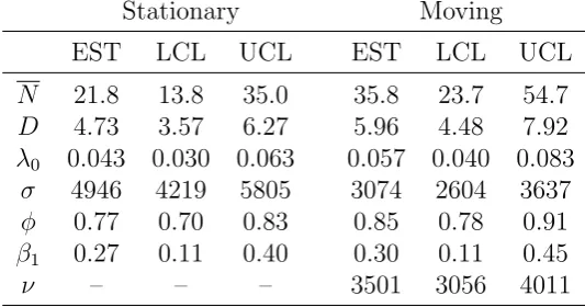
[Table 1 about here.]
The best fitting model selected by AIC had activity centers, encounter rate, and detection
range change by occasion while survival probability, recruitment rate, and movement
range were constant (Table 1). The covariate describing the technology used for each
camera (digital or not) did not provide a better or comparable fit (assessed by AIC)
compared to allowing detection probability to change for every occasion.
The best fitting model selected by AIC among models where activity centers were
stationary over time also had encounter rate and detection range vary by occasion while
Accepted
Article
3 APPLICATION: JAGUARS 3.3 Comparison with other methods
model and model with moving activity centers is shown in Figure 3. Table 1 shows the
maximum likelihood estimates from both models. There is a remarkable difference in the
estimated mean abundance: a 40% reduction in the estimated abundance when activity
centers are assumed to be stationary. Furthermore, the stationary model estimates
survival to be 10% lower and activity range to be 60% larger. The substantial effect
the assumption of stationary activity centers has on the resultant inference makes clear
that this assumption must be validated for any application of open population models.
Moving activity centers, when present in the survey but unaccounted for in the model,
leads to two problems. First, as individuals are seen over a wider range over the entire
survey compared to within each occasion, the stationary model compensates for this
by overestimating activity range and underestimating encounter rate; this ultimately
leads to an overestimation of detection probability and, in this case, a substantially
underestimated density. The second problem is while the model with movement is able
to account for reduced detectability due to movement, the stationary model cannot and
tends to explain this reduced detectability by lowering survivial probability: individuals
that move out of detectable range are best explained by having failed to survive.
One question is whether there is evidence that population density has changed over time.
To investigate this, one can consider the estimated rate of change in density between
occasions: ∆k = (Dk+1 − Dk)/∆tk where ∆tk is the time between occasions k and
k+ 1. Using the best-fitting model with moving activity centers, a parametric bootstrap,
simulating from the estimated asymptotic distributions of the parameters, is used to
estimate the variance of these differences. The mean change in density between occasions
was 0.06 individuals per 100 square kilometers with an estimated 95% confidence interval
of (−0.02,0.21) using 1000 bootstrap re-samples. As the estimated confidence interval
includes zero, this indicates that the evidence for population density changing over time
is not statistically significant.
[Figure 3 about here.]
3.3 Comparison with other methods
Two popular SCR alternatives to the HMM method presented here are closed-population
SCR and the Bayesian implementation of the open population models using data
aug-mentation. These methods were applied to the jaguar case study to compare resultant
inference and efficiency. For both methods, the same formulations for detection and, for
the Bayesian model, population dynamics were used as in the models above.
Accepted
Article
3.3 Comparison with other methods 3 APPLICATION: JAGUARS
be closed within the survey conducted each year and surveys across years assumed to
be independent. This means that if an individual was captured in separate years, this
information is ignored and the detections treated as if they are from distinct individuals.
Hence, one cannot explicitly estimate recruitment or survival probability. On the other
hand, as activity centers between years are unrelated, this model is robust to movement
between occasions. Separate detection and density parameters are estimated for each
year using standard SCR methods. Figure 3 shows that the open population model with
moving activity centers and the closed population approach provide similar inference
on trend over time; however, the trend in density is more noisy when estimated by
closed population SCR due to treating years separately. To mitigate this, density can
be described by a smooth, such as a cubic spline, over time. Closed-population models
were fitted with density constant or changing smoothly according to a regression spline
with increasing dimension and then compared by AIC. The best model describes density
as a constant over time with mean 2.33 individuals per 100 square kilometers and 95%
confidence interval (1.94,2.80). This is consistent with the open population model where
no statistically significant evidence is found for a change in density over time.
The closed population approach led to less precise estimates of density. The open
population model provides more precise estimates by using the additional information
that the closed population approach ignores. Applying a smooth to the closed
popula-tion estimates leads to similar precision to that from the open populapopula-tion model. The
primary advantage of the open population model over the closed population model is
the ability to make explicit inference about survival and recruitment probabilities from
the observations made on individuals during the survey.
The HMM approach was also compared to the Bayesian data augmentation approach
proposed in Gardner et al. (2010). The Bayesian method was implemented inrjags 4.6
(Plummer, 2013) with weakly informative priors. The posterior was approximated by
100,000 iterations with a burn-in of 5000 iterations for the stationary model and 20,000
for the model with moving activity centers. Inference obtained from the Bayesian method
was similar to that from the maximum likelihood HMM approach for both stationary
and moving activity center models (see Web Appendix D for the Bayesian results).
For the simplest model, all parameters being constant over time, maximum likelihood
inference was obtained in 5.5 minutes while the data augmentation took 23 hours. For
the best fitting models identified above, maximum likelihood inference took 4 hours to fit
compared to 1.5 days. Both methods were implemented on a desktop Intel(R) Core(TM)
Accepted
Article
4 SIMULATION STUDY
with data augmentation in JAGS, averaging over life history with R and Rcpp using
a HMM was more computationally efficient, provided similar inference, and avoided
auto-correlation issues common when MCMC is applied to models with latent temporal
processes. Some of this computational efficiency is gained from switching from using
JAGSto usingRcppand some from switching from data augmentation to marginalization.
The comparison, however, does show the relative efficiency of the maximum likelihood
analysis compared to the common, at present, JAGSanalysis conducted by practitioners.
4. Simulation study
The performance of the maximum likelihood estimators was investigated by simulation.
Surveys identical to the jaguar survey, with the same camera locations and number of
occasions, were simulated. All parameters were set to be constant over the survey with
λ0 = 0.05, σ = 3000, φ= 0.8, β1 = 0.2, andD= 0.06. Two scenarios were considered, one
where activity centers were stationary and one where they moved by Brownian motion
with standard deviation ν = 3000. For the stationary simulations, an open population
model with stationary activity centers and a closed population spatial capture-recapture
model were fit to each data set by maximum likelihood. For the simulation with moving
activity centers, two open population models were considered, one with a movement
model and one without, along with a closed population model. Percentage relative
bias and 95% confidence interval coverage was estimated for each parameter from one
thousand simulations.
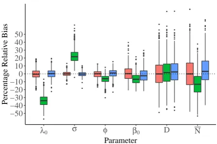
When activity centers are stationary, the model assuming stationary activity centers
is negligibly biased for all parameters (Figure 4) and 95% confidence interval
cov-erage is 94.6% on average for all parameters. When simulated activity centers move
between occasions, detection, survival, and recruitment parameters become notably
biased (Figure 4). Despite this, the estimated bias for the super-population density
remains small. This is similar to the findings of Royle et al. (2016): the stationary
model provides robust estimates of density by using the detection model to account
for the unobserved, unmodeled movement process: detection range is overestimated and
encounter rate underestimated. In the open population model, both the detection and
population dynamics models are distorted to account for the movement of individuals
in to, within, and out of the study area: initial recruitment probability, β1, and survival
probability are underestimated: individuals not present initially immigrate and some
present, emigrate.
Accepted
Article
5 CONCLUSION
estimated abundance (or density) within each occasion. As in the jaguar application, the
estimated density for each occasion is negatively biased when movement is not accounted
for. The within-occasion density estimator is biased because the population dynamics
(survival and recruitment) are confounded with the unmodeled movement process.
The open population model where movement is explicitly modeled provides estimates
that are negligibly biased (<3% in all cases) and confidence interval coverage was less
than one percent from nominal. For this scenario, β1 was marginally underestimated
and N marginally overestimated. This may indicate that at low sample sizes, moving
activity centers can still cause bias in the detection or population dynamics models due
to the subtle confounding between these processes.
When compared to the closed-population model fit to the same simulated data sets,
the mean percentage relative root-mean-square error in the estimate of density for each
occasion was on average 30% smaller for the open population model when compared
to the closed population model. Confidence intervals for the density on each occasion
were on average 2.5 times wider using the closed population model compared to the
open population model. The root-mean-square error and uncertainty in density
estima-tors from the closed population model could be reduced using a smoothing approach.
When smoothed, closed population models can provide similar inference on the trend in
population density, but not the mechanisms that drive these trends.
[Figure 4 about here.]
5. Conclusion
Formulating open population spatial capture-recapture (SCR) as a hidden Markov model
(HMM) incorporates CJS and JS models into a general framework and allows
marginal-ization over life histories and movement to be achieved with computational efficiency,
making more complex modeling and model selection practically feasible. Maximum
likelihood estimation leads to similar inference compared with a data augmentation,
Bayesian approach; furthermore, marginalization could be used in the Bayesian context
with a semi-complete data likelihood (King et al., 2016). Overall, the presented
frame-work is flexible and open to extension: alternative movement models, life histories with
more states (e.g.temporary emigration), and incorporation of observed states (i.e.dead
Accepted
Article
5 CONCLUSION
Acknowledgements
The authors thank the associate editor and two anonymous reviewers for their insightful
comments that led to an improved paper. David Borchers was part-funded by EPSRC
grant EP/K041061/1 and Richard Glennie was funded by the Carnegie Trust.
References
Borchers, D. L. and Efford, M. (2008). Spatially explicit maximum likelihood methods
for capture–recapture studies. Biometrics 64,377–385.
Calhoun, J. B. and Casby, J. U. (1958). Calculation of home range and density of small
mammals. Number 55. US Department of Health, Education, and Welfare, Public
Health Service.
Chandler, R. B. and Clark, J. D. (2014). Spatially explicit integrated population models.
Methods in Ecology and Evolution 5,1351–1360.
Cormack, R. (1964). Estimates of survival from the sighting of marked animals.
Biometrika 51,429–438.
Efford, M. (2004). Density estimation in live-trapping studies. Oikos 106, 598–610.
Efford, M. (2012). secr: Spatially explicit capture–recapture models. R package version
3.2.0.
Fewster, R. and Jupp, P. (2009). Inference on population size in binomial detectability
models. Biometrika 96,805–820.
Gardner, B., Reppucci, J., Lucherini, M., and Royle, J. A. (2010). Spatially explicit
inference for open populations: estimating demographic parameters from
camera-trap studies. Ecology 91,3376–3383.
Harmsen, B. J., Foster, R. J., Sanchez, E., Gutierrez-Gonz´alez, C. E., Silver, S. C., Ostro,
L. E., et al. (2017). Long term monitoring of jaguars in the Cockscomb Basin wildlife
sanctuary, Belize; implications for camera trap studies of carnivores. PloS one 12,
e0179505.
Harmsen, B. J., Foster, R. J., Silver, S. C., Ostro, L. E., and Doncaster, C. P. (2010). The
ecology of jaguars in the Cockscomb Basin wildlife sanctuary, Belize. The biology
and conservation of wild felids pages 403–416.
Jolly, G. M. (1965). Explicit estimates from capture-recapture data with both death
and immigration-stochastic model. Biometrika 52,225–247.
King, R., McClintock, B. T., Kidney, D., and Borchers, D. L. (2016). Capture-recapture
abundance estimation using a semi-complete data likelihood approach. Annals of
Accepted
Article
6 SUPPORTING INFORMATION
Otis, D. L., Burnham, K. P., White, G. C., and Anderson, D. R. (1978). Statistical
inference from capture data on closed animal populations. Wildlife monographs
pages 3–135.
Plummer, M. (2013). rjags: Bayesian graphical models using MCMC. R package version
3,.
Pollock, K. H. (1982). A capture-recapture design robust to unequal probability of
capture. The Journal of Wildlife Management46, 752–757.
R Core Team (2017). R: A Language and Environment for Statistical Computing. R
Foundation for Statistical Computing, Vienna, Austria.
Royle, J. A., Chandler, R. B., Sollmann, R., and Gardner, B. (2013). Spatial
capture-recapture. Academic Press.
Royle, J. A., Fuller, A. K., and Sutherland, C. (2016). Spatial capture–recapture models
allowing markovian transience or dispersal. Population ecology 58,53–62.
Schwarz, C. and Arnason, A. (1996). A general methodology for the analysis of
capture-recapture experiments in open populations. Biometrics 52,860–873.
Seber, G. A. (1965). A note on the multiple-recapture census. Biometrika 52,249–259.
Zucchini, W., MacDonald, I. L., and Langrock, R. (2016). Hidden Markov models for
time series: an introduction using R, volume 150. CRC press.
6. Supporting Information
Web Appendices referenced in Sections 2.5, 3.2, and 3.3 are available with this paper at
the Biometrics website on Wiley Online Library. Also, the R (R Core Team, 2017)
Accepted
Article
FIGURES FIGURES
Accepted
Article
[image:21.595.101.328.336.497.2]FIGURES FIGURES
Accepted
Article
FIGURES FIGURES
0.5 1 1.5 2 2.5 3 3.5 4 4.5 5 5.5 6 6.5
1 2 3 4 5 6 7 8 9 10 11 12 Occasion
Estimated Density
Accepted
Article
FIGURES FIGURES ● ● ● ● ● ● ● ● ● ● ● ● ● ● ● ● ● ● ● ● ● ● ● ● ● ● ● ● ● ● ● ● ● ● ● ● ● ● ● ● ● ● ● ● ● ● ● ● ● ● ● ● ● ● ● ● ● ● ● ● ● ● ● ● ● ● ● ● ● ● ● ● ● ● ● ● ● ● ● ● ● ● ● ● ● ● ● ● ● ● ● ● ● ● ● ● ● ● ● ● ● ● ● ● ● ● ● ● ● ● ● ● ● ● ● ● ● ● ● ● ● ● ● ● ● ● ● ● ● ● ● ● ● ● ● ● ● ● ● ● ● ● ● ● ● ● ● ● ● ● ● ● ● ● ● ● ● ● ● ● ● ● ● ● ● ● ● ● ● ● ● ● ● ● ● ● ● ● ● ● ● ● ● ● ● ● ● ● ● ● ● ● ● ● ● −50 −40 −30 −20 −10 0 10 20 30 40 50λ0 σ φ β0 D N
Parameter
Percentage Relativ
[image:23.595.212.436.290.439.2]e Bias
Figure 4. Boxplot of relative percentage bias from one thousand simulated open population spatial capture-recapture surveys for encounter rate λ0, detection range σ,
survival probability φ, probability an individual is present at the start of the survey
β1, super population density D, and mean abundance on a single occasion N in the
Accepted
Article
[image:24.595.160.427.199.339.2]TABLES TABLES
Table 1
Maximum likelihood estimates (EST), lower (LCL) and upper (UCL)95%confidence intervals from open population spatial capture-recapture models for mean abundance within a single occasion (N), density of super-population (D), mean encounter rate (λ0), mean activity range (σ), survival probability (φ), probability alive at the start of the survey (β1), and standard deviation of movement of activity centers (ν). Estimates are
for the best fitting models (selected by AIC) where activity centers were stationary over time (left) and where activity centers were moving according to Brownian motion (right).
Stationary Moving
EST LCL UCL EST LCL UCL
N 21.8 13.8 35.0 35.8 23.7 54.7
D 4.73 3.57 6.27 5.96 4.48 7.92
λ0 0.043 0.030 0.063 0.057 0.040 0.083
σ 4946 4219 5805 3074 2604 3637
φ 0.77 0.70 0.83 0.85 0.78 0.91
β1 0.27 0.11 0.40 0.30 0.11 0.45