Bayesian Approach to Ranking and Selection for a Binary Measurement System

(1)

ISSN Print: 2161-718X

DOI: 10.4236/ojs.2019.94029 Aug. 13, 2019 436 Open Journal of Statistics

Bayesian Approach to Ranking and

Selection for a Binary Measurement System

Mark Eschmann

1

_{, James D. Stamey}

2

_{, Phil D. Young}

3

_{, Dean M. Young}

4

1_{Department of Statistical Science, Waco, TX, USA}

2_{Department of Statistical Science, Baylor University, Waco, TX, USA} 3_{Department of Information Systems, Baylor University, Waco, TX, USA} 4_{Department of Statistical Science, Baylor University, Waco, TX, USA}

Abstract

Binary measurement systems that classify parts as either pass or fail are wide-ly used. Inspectors or inspection systems are often subject to error. The error rates are unlikely to be identical across inspectors. We propose a random ef-fects Bayesian approach to model the error probabilities and overall con-forming rate. We also introduce a feature-subset selection procedure to de-termine the best inspector in terms of overall classification accuracy. We pro-vide simulation studies that demonstrate the viability of our proposed estima-tion ranking and subset-selecestima-tion methods and apply the methods to a real data set.

Keywords

Bayesian Statistics, Quality Control, Binary Measurement Systems, Misclassification

1. Introduction

Repeated binary testing, often referred to as a binary measurement system (BMS), is regularly used in quality control studies as a means of assessing the quality of the units produced. However, these inspection methods are highly de-pendent on the quality of the individual inspectors, thus making the inspection itself an integral part of the quality control process. Two aspects of evaluating the inspection process are repeatability and reproducibility. A process’s repeata-bility refers to how frequently a single inspector inspecting a single item will ob-tain the same result, while reproducibility refers to how often different inspec-tors inspecting the same item will reach the same conclusion. Estimating classi-fication rates of a system has been considered by several authors. [1] considered

How to cite this paper: Eschmann, M., Stamey, J.D., Young, P.D. and Young, D.M. (2019) Bayesian Approach to Ranking and Selection for a Binary Measurement Sys-tem. Open Journal of Statistics, 9, 436-444.

https://doi.org/10.4236/ojs.2019.94029

Received: June 25, 2019 Accepted: August 10, 2019 Published: August 13, 2019

http://creativecommons.org/licenses/by/4.0/

(2)

DOI: 10.4236/ojs.2019.94029 437 Open Journal of Statistics

various sampling plans to assess the qualities of a BMS. [2] found maximum li-kelihood estimators and method of moment estimators for the case of multiple raters, assuming fixed effects. When there are multiple inspectors, it may be of interest to determine which of several inspectors or inspection systems is per-forming best.

The model we consider here is a Bayesian version of [3]. Specifically, we con-sider a random effects model for multiple testers and multiple inspections per inspector from a Bayesian perspective. There are multiple advantages to using a Bayesian approach. For example, prior knowledge can be incorporated into the study with the use of informative prior distributions. This knowledge can be ob-tained either from previous data or expert opinion. Also, even in the absence of prior knowledge where the asymptotic dominance of the prior by the likelihood is present, interval estimates generated from the Bayesian paradigm are based largely on the likelihood which has been shown to be superior to other interval estimation methods [4]. Another advantage of the Bayesian paradigm is that if the prior is sufficiently informative, then, assumptions required for identifiabili-ty can be relaxed. Thus, our Bayesian approach can be used in situations when the parameters of a likelihood function are not identifiable. The Bayesian esti-mators considered here have no known closed form and, thus, must be found approximately. We use Markov Chain Monte Carlo (MCMC) simulations to sample from the model’s posterior distribution and obtain parameter estimates.

The remainder of the paper is outlined as follows. In Section 2, we present the model and give identifiability assumptions. In Section 3, we describe a simula-tion study and present the simulasimula-tion results for the Bayesian estimasimula-tion. In Sec-tion 4, we apply our model to two parameter-ranking applicaSec-tions and two sub-set selection problems for multiple sites, and in Section 5, we perform an addi-tional simulation to determine the effectiveness of our subset selection proce-dure. Finally, in Section 6, we provide several comments summarizing our re-sults.

2. The Model

Assume that N randomly selected items to be inspected are sampled from the general population of items. Let the true quality state of an item be denoted by T, where T =1_{indicates a good item and}T =0_{denotes an item that fails to}

meet the quality specifications. The symbol

τ

_{denotes the overall conforming}

rate. Because we assume that no gold standard is used and because T is a latent variable, we also assume T ~ Bernoulli

( )

τ _.

Repeated independent, fallible observations are then derived by m different inspectors on the ith_{unit to indirectly assess the true state of the}_ith_{unit, where}

{

1, ,

}

i∈ _ N _{. Let}Y_ijk denote the result of the kth_{inspection on the}_ith_{item by}

the jth_{inspector, where} ₁

ijk

Y = _{denotes a passed inspection,}Yijk =0 denotes a

failed inspection, and k∈

{

1, , nij

}

. For each Yijk and inspector j, we further

define the conditional probabilities

θ

j,+=P Y

(

ijk =1|Ti =0

)

(false positive rate)

(3)

the item, Ti. Further, assume

(

Y Tijk| i=0 ~ Bernoulli

)

( )

θj,+ (1)

and

(

Y Tijk| i=1 ~ Bernoulli 1

)

(

−θj,−

)

. (2)

here, we initially assume that inspections are independent, given the true latent state of the ith_{part. This conditional independence assumption yields}

(

,

)

1 | 0 ~ Binomial , .

l

ijk i j

k Y T l

θ + =

 ₌ 

 



∑

 (3)

To relax assumptions that the inspectors all have the same probability of clas-sifying correctly and allow for other random heterogeneity, we consider the random effects model where

(

)

(

)

,

~ Beta , , ~ Beta , , j

j

θ µ γ

+ + +

− − −

(4)

where the Beta distribution has been reparameterized such that µ α α β=

(

+

)

and

γ α β

= + _{. Thus, the reparameterized Beta probability density function}

(PDF) is

( )

₍

1

(

1

)

₎

1.

, x x f x B γ µγ µγ

µγ γ µγ

− −

− ₋

=

− (5)

To complete the hierarchical model we require priors for µ₊_, µ₋_, γ₊_and γ−. Specifically we assume Beta

(

α β+, +

)

and Beta

(

α β−, −

)

priors for µ+

and µ₋_{, respectively. Finally,} Gamma

₍

c d+, +

₎

and Gamma

(

c d−, −

)

priors are

used for γ+ and γ− , respectively. In the absence of prior information,

( )

Beta 1,1 priors can be used for µ₊_and µ₋_{and diffuse Gamma priors are}

used for γ+ and γ−.

We have chosen a Beta distribution to model the random effects because of its interpretability under this reparameterization. An often used alternative model structure is

( )

(

)

logit θ ~ N µ σ, , (6) where

µ

is generally given a normal prior and σ is often given a half-t or half-Cauchy prior.

For the parameters Θ=

{

θ θ₋, ₊

}

_and Ψ:=

{

µ γ µ γ τ₊, , , ,₊ ₋ ₋

}

_{, the likelihood}

of the latent vector t=

[

t1, ,tN

]

′, the observed data matrix is X =

[

x1′, , xN′

]

′,

where x= xi,1, , xi m, ′ and

(

)

(

) (

)

(

)

(

)

( )

(

)

( )( ) 1 1 1 1 1 1 1 1

1 1 1

1 1 1 , , | | , , , | 1 1 1 . N N

N _i _i _{i ij}

i i

i

N N

i ij ij i ij

i i

N

i ij ij i

m _{t x}

N t

t

j j

m

t n x t x

j j

j

t n x

j

f f f

µ γ

γ µ γ µ γ

γ µ γ

τ τ θ

θ θ θ − − = = = − − − + + = = + + + = + − − − = − + − − − + − − + = − − + − − + ∑ ∑ ∑ ∑ ∑ ∑ =  = − _ −    ×    × − _ 

∏

x t Θ Ψ x t ΘY t Θ Ψ

(4)

For the random effects model, the first assumption necessary for identifiability

[3] is

1.

µ₊+µ₋< ₍₈₎

The interpretation of (8) is that the overall expected probability of correctly classifying an item is greater than the chance of misclassifying it. This assump-tion is required due to the bimodal nature of the likelihood [4].

The second identifiability assumption assures that there are enough degrees of freedom to estimate all model parameters. This assumption requires two things: that enough inspectors and inspections per inspector are available to estimate the status of each item, and that enough inspectors are available to estimate the inspectors’ random effects parameters. The second condition requires at least two inspectors while letting lj=min

(

nij, , nNj

)

. A sufficient condition to

meet the first requirement is that

(

)

1

1 m j 1 2 1.

j= l m

− +

∏

+ ≥ + ₍₉₎

In the present model, (9) is sufficient because additional inspections do not harm the model identifiability.

The third identifiability assumption is that both true negatives (Ti =0) and

true positives (Ti=1) exist in the sample. This assumption is necessary because

the absence of true negatives indicates one cannot estimate false negative rates.

[3] have demonstrated that the absence of either true negatives or true positives essentially implies that there is enough data to estimate only half of the variables, namely θ₊_, µ₊_{, and}γ₊_orθ₋_, µ₋_{, and}γ₋_{. We remark that the last two}

identifiability requirements can be omitted if one uses sufficiently informative priors on at least some parameters.

3. Ranking and Selecting Inspectors

Suppose we are interested in determining which inspector has the lowest overall error rate. Here, we have chosen to combine the false positive and false negative rates into a single positive likelihood ratio (LR),

η

j = −

(

1

θ

j,+

)

θ

j,−. Whichever

inspector has the highest likelihood ratio would be determined to be the best. The positive likelihood ratio may not always be the most appropriate combina-tion of the error rates, however, it is simply the one we use here as an example. In some cases, the negative likelihood ratio,

η

j =

θ

j,+

(

1−

θ

j,−

)

or even a

weighted sum of θ+ and θ− may be more appropriate. This approach can be

decided on a case by case basis. We follow the method of [5] who have derived a decision-theoretic approach to partition parameters into two sets based on an ordering of the parameters of interest. Also, [6] extended their work to deter-mine the largest Poisson rate when counts are subject to misclassification. Here we apply the method to subset a group of inspectors into a superior set, S, and an inferior set, _SC_.

(5)

prob-DOI: 10.4236/ojs.2019.94029 440 Open Journal of Statistics

lems. Each decision involves whether or not to place an inspector’s likelihood ratio in the superior set, k :

k

d+ η ∈S. We assign following constant loss

func-tions:

( )

2

1

0 if if

and

if k best 0 if k best

k k

k best k best

c

L L

c

η η η η

η η

η η η η

+ −

= =

 

=_ =_

≠ ≠

  (10)

where _Lk

+ and Lk− are the loss functions for d+k and d−k, respectively. To

make a decision, only c c c= 2 1 is required. These loss functions determine the

decision criteria: take action _dk

+ and include ηk as a candidate for the largest

parameter if P

(

ηk =ηbest|x

)

≥1

(

c+1

)

. Here, generally, c2>c1 because

fail-ing to place the best ηk in S is the more serious error. Thus, c should be chosen

larger than 1.

The probability that ηk is the best of the likelihood ratios is

(

)

1

(

)

1 1 1

0 0 0

| i i | d d d d d ,

i best i i m i

P η η= x =

_{∫ ∫}

η

_∫

ηp η x η η₋ η₊  η η (11) where p

(

η|x

)

is the marginal posterior of the likelihood ratios. MCMC me-thods are used to approximate (11) numerically. To accomplish this task, we generate a sample

(

η η

k1, k2, ,

η

kB

)

′, for k=1,2, , m of size B from the

post-erior distribution, and then approximate the postpost-erior probability that ηk is the

best parameter by

(

)

(

)

(

1

)

1

# , ,

ˆ _{, ,} _| ki i mi _,

k m

best

P best

B

η η η

η = η η x = =  (12)

where k=1, ,_ m_and

i

=

1,2, ,



B

, and B is the Monte Carlo repetition size. The parameter ηk is included in the superior set S if

(

)

(

1

)

(

)

ˆ _k _{, ,} _m _| ₁ _{1 ,} _{1, , .}

P

η

=best

η



η

x ≥ c+ k=  m (13)

4. Example

As an example we consider data from [4] on a sample of 38 prints produced by inkjet cartridges. Three inspectors analyzed each print 3 times. Only the total number of passes out of the 9 inspections was provided, so for illustrative pur-poses, for those parts that did not have 0 or 9 passes, we distributed the number of passes across the three inspectors in a way to best match the frequentist pa-rameter estimates provided in [4]. We assign beta (1, 9) priors to both µ+ and

µ₋_{since both of these quantities are expected to be considerably below 0.50.}

Our expert was 95% certain that both misclassification rates were less than 0.40, and a beta (1, 9) prior appropriately modeled the uncertainty. These distribu-tions have prior 95% intervals of (0.003, 0.336) and have an equivalent sample size of 10 observations, and, therefore, would be considered mildly informative. A beta (1, 1) prior is used for

τ

, and Gamma (0.1, 0.1) priors are used for both

γ+ and γ−. A burn-in of 10,000 iterations was used and inferences were based

(6)

[image:6.595.209.539.89.317.2]

Table 1. Posterior summary for [4] example.

Post.Median Post.SD val2.5pc val97.5pc

µ− 0.07818 0.06041 0.01913 0.251

µ+ 0.126 0.06176 0.04415 0.2841

γ− 4.423 6.154 0.5477 22.93

γ+ 7.836 8.252 1.183 31.93

1

θ− 0.08885 0.03579 0.03632 0.1776

2

θ₋ _0.001537 _0.01049 _2.20E-06 _0.03754

3

θ− 0.03101 0.02175 0.005326 0.08751

1

θ− 0.04653 0.03027 0.009797 0.1253

2

θ− 0.1283 0.04255 0.06432 0.2303

3

θ− 0.148 0.04656 0.07318 0.2543

1

η _19.52 _32.73 _7.21 _92.31

2

η 7.746 2.995 4.31 15.45

3

η 6.525 2.471 3.798 13.19

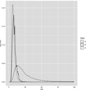
From Figure 1, we see that when combined into the positive likelihood ratio, where a higher number is better, Inspector 1 has the overall highest LR. To apply the decision theoretic procedure to determine if any inspector is “best,’’ we compute the posterior probabilities of each likelihood ratio parameter being the largest. Here, a value of c=10, implies that it is 10 times worse to leave the best inspector out of the superior set than to put an inferior inspector in the superior set, the critical probability would then be 1/(10 + 1) = 0.091. The probabilities that Inspectors 1, 2, and 3 are each in the superior set are 0.891, 0.083, and 0.026, respectively. Thus, here, only Inspector 1 exceeds the 0.091 probability threshold. Thus, inspector 1 would be the only inspector placed in the superior set.

5. A Simulation Study

We conducted a simulation study to determine the effectiveness of the subset selection procedure. We set the number of inspectors to be m=7_{and the}

number of repeats to be l=3. For τ =0.5, µ+ =0.15, µ−=0.1, γ+ =20,

and γ₋=40_{we generated a single set of}θ₊_,_j_{’s and}θ₋_,_j_{’s. The values for}θ₊_,_j_,

,j

θ− and the corresponding likelihood ratios are presented in Table 2.

The prior distributions used were

( )

~beta 1,1 ,

µ₊ ₍₁₄₎

( )

~beta 1,1 ,

µ₋ (15)

(

)

~Gamma 0.1,0.1 ,

γ+ (16)

(

)

~Gamma 0.1,0.1 ,

γ₋ ₍₁₇₎

and

( )

~beta 1,1 .

(7)

[image:7.595.230.516.70.367.2]

[image:7.595.209.539.418.554.2]

Figure 1. Posterior distributions of likelihood ratios.

Table 2. Misclassification parameters for simulation study.

Inspector θ− θ+ LR

1 0.014 0.09 10.96

2 0.084 0.218 4.20

3 0.094 0.119 7.60

4 0.224 0.168 4.62

5 0.175 0.153 5.39

6 0.033 0.076 12.72

7 0.02 0.105 9.33

Table 3. Simulation results for N=50.

Inspector P

(

η ηk= best

)

2.5% Median 97.5%

1 0.29 1.05 2.59 5.16

2 0.01 3.34 5.77 6.98

3 0.09 1.43 3.8 6.3

4 0.01 2.91 5.55 6.97

5 0.03 2.39 5.06 6.87

6 0.37 1.01 2.29 4.89

[image:7.595.209.539.586.729.2]

(8)

[image:8.595.210.540.90.226.2]

Table 4. Simulation results for N=100_.

Inspector P

(

η ηk= best

)

2.5% Median 97.5%

1 0.31 1.06 2.22 4.08

2 0 4.66 6.23 6.98

3 0.05 1.84 3.73 5.55

4 0 4.15 5.9 6.94

5 0 3.39 5.24 6.72

6 0.47 1.01 1.88 3.72

7 0.16 1.24 2.79 4.65

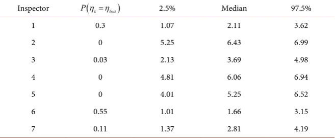
Table 5. Simulation results for N=200.

Inspector P

(

η ηk= best

)

2.5% Median 97.5%

1 0.3 1.07 2.11 3.62

2 0 5.25 6.43 6.99

3 0.03 2.13 3.69 4.98

4 0 4.81 6.06 6.94

5 0 4.01 5.25 6.52

6 0.55 1.01 1.66 3.15

7 0.11 1.37 2.81 4.19

Thus, relatively non-informative priors were employed for all parameters. We considered sample sizes of N=50_{, 100, and 200 and generated 1000 data sets}

for each sample size. We monitored the probability that each likelihood ratio is the largest and the 95% credible set of the rank for each ηi. These results are

provided in Tables 3-5. For the decision theory problem we used c=10_and,

thus, also monitored whether the true “best’’ inspector was included in the supe-rior set as well as the average size of the supesupe-rior set. In this paper we are focus-ing on the rankfocus-ing and selection methods, so those are the simulation results we report here. We also monitored posterior means and found they were close to the true values with small bias and coverage of intervals close to nominal for all parameters. The bias and coverage results are available upon request.

For all simulations, Inspector 6, who was the “best’’ inspector, yielded the highest probability of having the largest likelihood ratio, and, therefore, was correctly estimated to be the best inspector the most times. Also, the credible in-tervals on the ranks for Inspector 6 were consistently closest to the top rank. Conversely, Inspector 2, who was the “worst’’ inspector, produced the lowest probability of having the largest likelihood ratio and, was correctly considered the worst inspector the most times. Inspector 2 also yielded credible intervals for the rank with the largest values, implying this inspector was generally ranked last. Thus both the ranking and selection procedures performed well.

[image:8.595.210.539.259.395.2]

(9)

being included in the superior set was greater than 0.9. The average size of the superior set was 2.8 for a sample size of 50, 2.4 for a sample size of 100 and 2.2 for a sample size of 200.

6. Conclusions

In this paper we have proposed a Bayesian random effects model for a binary measurement system. As shown in our real data example, combining the data with mildly informative priors yields an identifiable model where inferences can be made on the overall classification rates along with comparisons of individual inspectors. Our simulation study shows that for moderate sample sizes, even when information is not available for priors, the procedure works well with the best inspector being included in the superior set a large percentage of the time.

The methods we have proposed could be extended to comparing overall de-fective rates and classification probabilities of manufacturing plants instead of inspectors, as we have done here. Expanding to continuous measurements from binary is also potentially of interest.

Conflicts of Interest

The authors declare no conflicts of interest regarding the publication of this pa-per.

References

[1] Danila, O., Steiner, S.H. and MacKay, R.J. (2008) Assessing a Binary Measurement System. Journal of Quality Technology, 40, 310-318.

https://doi.org/10.1080/00224065.2008.11917736

[2] van Wieringen, W.N. (2008) Measurement System Analysis for Binary Data. Tech-nometrics, 50, 468-478.https://doi.org/10.1198/004017008000000415

[3] Danila, O., Steiner, S.H. and MacKay, R.J. (2012) Assessing a Binary Measurement System with Varying Misclassification Rates Using a Latent Class Random Effects Model. Journal of Quality Technology, 44, 179-191.

https://doi.org/10.1080/00224065.2012.11917894

[4] Boyles, R.A. (2001) Gauge Capability for Pass-Fail Inspection. Technometrics, 43, 223-229.https://doi.org/10.1198/004017001750386332

[5] Bratcher, T.L. and Bhalla, P. (1974) On the Properties of an Optimal Selection Pro-cedure. Communications in Statistics: Simulation and Computation, 3, 191-196.

https://doi.org/10.1080/03610927408827118

[6] Stamey, J.A., Bratcher, T.L. and Young, D.M. (2004) Parameter Subset Selection and Multiple Comparisons of Poisson Rate Parameters with Misclassification. Compu-tational Statistics & Data Analysis, 45, 467-479.