Numerical Analysis for Kinetics of Reactive Diffusion Controlled by Boundary and Volume Diffusion in a Hypothetical Binary System

Numerical Analysis for Kinetics of Reactive Diffusion Controlled by Boundary

and Volume Diffusion in a Hypothetical Binary System

Akira Furuto

and Masanori Kajihara

1

Graduate School, Tokyo Institute of Technology, Yokohama 226-8502, Japan

2_{Department of Materials Science and Engineering, Tokyo Institute of Technology, Yokohama 226-8502, Japan}

A hypothetical binary system composed of one intermetallic compound and two primary solid-solution phases has been considered in order to examine the kinetics of the reactive diffusion controlled by boundary and volume diffusion. If a semi-infinite diffusion couple initially consisting of the two primary solid-solution phases with solubility compositions is isothermally annealed at an appropriate temperature, the compound layer will be surely produced at the interface between the primary solid-solution phases. In the primary solid-solution phases, however, there is no diffusional flux. Furthermore, we suppose that the compound layer is composed of a single layer of square-rectangular grains with an identical dimension. Here, the square basal-plane is parallel to the interface, and hence the height is equal to the thickness of the compound layer. Under such conditions, the growth behavior of the compound layer has been analyzed numerically. In order to simplify the analysis, the following assumptions have been adopted for the compound layer: there is no grain boundary segregation; and volume and boundary diffusion takes place along the direction perpendicular to the interface. When the size of the basal-plane remains constant independently of the annealing time, the thickness of the compound layer is proportional to the square root of the annealing time. In contrast, the growth of the compound layer takes place in complicated manners, if the size of the basal-plane increases in proportion to a power function of the annealing time. Nevertheless, around a certain critical annealing time, the thickness of the compound layer is approximately expressed as a power function of the annealing time. For each grain, the layer growth is associated with increase in the height, and the grain growth is relevant to increase in the size of the basal-plane. The exponent for the layer growth almost linearly decreases with increasing exponent for the grain growth. [doi:10.2320/matertrans.MRA2007192]

(Received August 6, 2007; Accepted November 12, 2007; Published December 27, 2007)

Keywords: diffusion, kinetics, modeling

1. Introduction

The growth behavior of intermetallic compounds during reactive diffusion has been experimentally observed for various alloy systems by many investigators.1–27)_{In such an} experiment, a semi-infinite diffusion couple consisting of different pure metals or alloys may be isothermally annealed at an appropriate temperature. Owing to annealing, some of the stable compounds will be formed as layers at the interface in the diffusion couple. If the growth of the compound layers is controlled by volume diffusion, a parabolic relationship holds good between the total thickness of the compound layers and the annealing time. Here, the parabolic relation-ship means that the total thickness is proportional to the square root of the annealing time. However, volume diffusion is not necessarily the rate-controlling process of reactive diffusion for all the alloy systems.

The kinetics of the reactive diffusion in the binary Au-Sn system was experimentally observed using Sn/Au/Sn dif-fusion couples at solid-state temperatures in previous studies.28–31) _{In those experiments, the diffusion couples} were isothermally annealed at temperatures between T¼ 393and 473 K for various times in an oil bath with silicone oil. Here,T is the annealing temperature. Due to annealing, compound layers of AuSn, AuSn2and AuSn4are produced at the Au/Sn interface in the diffusion couple. According to the observation, the total thickness of the Au-Sn compound layers is mathematically expressed as a power function of the annealing time, and the exponent of the power function is 0.48, 0.42, 0.39 and 0.36 at T ¼393, 433, 453 and 473 K, respectively. Such temperature dependence of the exponent

indicates that boundary diffusion as well as volume diffusion contributes to the rate-controlling process and grain growth occurs in the compound layers at certain rates at higher annealing temperatures.30) _{As the annealing temperature} decreases, the contribution of the boundary diffusion be-comes more remarkable, but the grain growth slows down. This is the reason why the exponent is smaller than 0.5 at higher annealing temperatures but close to 0.5 at lower annealing temperatures. The reactive diffusion controlled by boundary and volume diffusion takes place in many alloy systems.28–45) _{The rate-controlling process of such reactive} diffusion is hereafter called the mixed rate-controlling process.

The kinetics of the mixed rate-controlling process was theoretically analyzed using a mathematical model by Farrell and Glimer.34) In their model, a polycrystalline compound layer consisting of tabular grains with an identical width and flat grain boundaries with a certain thickness is formed at the interface between solid-solution phases with solubility compositions in a semi-infinite diffusion couple. Here, each tabular grain is sandwiched between the parallel grain boundaries perpendicular to the interface. During growth of the compound layer, one-dimensional boundary diffusion takes place along the grain boundary, and two-dimensional volume diffusion occurs along the directions perpendicular to the grain boundary and the interface. However, no diffusional flux exists in the solid-solution phases. Under such con-ditions, the growth behavior of the compound layer was calculated numerically. The numerical calculation was carried out mainly for the growth of the compound layer without grain growth. According to the calculation, the thickness of the compound layer increases in proportion to a power function of the annealing time, and the exponent of the

*_{Corresponding author, E-mail: [email protected]}

power function takes a constant value of 0.48. Thus, the exponent is slightly smaller than 0.5. In order for the compound layer to grow continuously, solute atoms should be transported along the grain boundary over long distances. However, the solute atoms in the grain boundary will be partially wasted due to the volume diffusion along the direction perpendicular to the grain boundary. Such partial wastage of the solute atoms slightly decelerates the growth of the compound layer. This is the reason why the exponent is slightly smaller than 0.5.

The growth of a compound layer controlled by boundary diffusion was theoretically analyzed using a different model by Corcoran et al.35) In their model of a semi-infinite diffusion couple, a polycrystalline compound layer is composed of cylindrical grains with an identical diameter, where the rotation axis of the grain is perpendicular to the interface and the diameter of the grain is expressed as a power function of the annealing time. Unlike the model by Farrell and Glimer,34)_{only boundary diffusion takes place in} the compound layer, but volume diffusion occurs merely in the neighboring phase ahead of the growing compound layer. If the contribution is much greater for the boundary diffusion than for the volume diffusion, the thickness of the compound layer is proportional to a power function of the annealing time.35)_{Furthermore, the exponent of the power function is} much smaller than 0.5 on condition that grain growth considerably occurs in the compound layer. Such conclusions may be drawn also for the mixed rate-controlling process with grain growth. Unfortunately, however, reliable infor-mation of the kinetics is not available for this type of mixed rate-controlling process. In order to examine the influence of grain growth on the kinetics of the mixed rate-controlling process, the growth behavior of a polycrystalline compound layer in a semi-infinite diffusion couple initially composed of solid-solution phases has been numerically analyzed in the present study. Here, the compound layer consists of a single layer of square-rectangular grains with an identical size, and volume and boundary diffusion occurs across the compound layer. However, it is assumed that there is no diffusional flux in the solid-solution phases. This assumption emphasizes the influence. The kinetics has been quantitatively discussed on the basis of the numerical analysis.

2. Model

Let us consider a hypothetical binary A-B system composed of two primary solid-solution phases and one intermetallic compound. Hereafter, the A-rich and B-rich solid-solution phases are called the and phases, respectively, and the intermetallic compound is designated the phase. For such a binary system, we consider a semi-infinite diffusion couple consisting of theandphases with initial compositions of c _{andc, respectively. Here,cis} the concentration of component B measured in mol per unit volume, andcandccorrespond to the composition of the phase for the=tie-line and that of thephase for the= tie-line, respectively, in the phase diagram of the binary A-B system. The semi-infinite diffusion couple means that the thicknesses of theand phases are semi-infinite and the = interface is flat. In such a diffusion couple, the

interdiffusion of components A and B occurs unidirectionally along the direction perpendicular to the flat interface. This direction is hereafter called the diffusional direction. When the diffusion couple is isothermally annealed at temperature

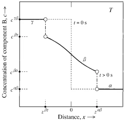
Tfor an appropriate time, thephase will be produced at the interface owing to the reactive diffusion between theand phases. Here, T is high enough for the reactive diffusion to occur sufficiently fast but lower than the temperature at which the liquid phase is stable. The concentration profile of component B across the phase along the diffusional direction is drawn in Fig. 1. In this figure, the ordinate shows the compositionc, and the abscissa indicates the distancex

measured from the initial position of the = interface. Dashed lines and solid curves show the concentration profiles before and after annealing, respectively, and z _{and z} indicate the positions of the = and = interfaces, respectively, after annealing. If the local equilibrium is realized at each migrating interface during annealing, the compositions of the neighboring phases at the interface coincide with those of the corresponding tie-line at temper-atureT. Such a reaction will actually proceed on condition that the interface diffusion across the migrating interface is much faster than the interdiffusion across the compound layer. In this case, the migration of the interface is controlled by the interdiffusion. This type of reaction is usually denominated the diffusion-controlling reaction. For the diffusion-controlling reaction, the migration rates dz_=dt anddz_{=dtof the=and= interfaces, respectively, are} related to the flux balance at the interface by the equations46)

ðccÞdz

dt ¼J

ð1aÞ

and

ðccÞdz

dt ¼ J

_{; ð1bÞ}

respectively. Here,J andJ are the diffusional fluxes of component B in thephase at the =and= interfaces, respectively. According to Fick’s first law, the diffusional Fig. 1 Concentration profile of component B across thephase in the

fluxes J and J are proportional to the concentration gradientsð@c_=@xÞ

x¼zandð@c=@xÞ_x¼zin thephase at the

=and=interfaces, respectively, as follows:

J¼ D @c

@x

x¼z

ð2aÞ

and

J¼ D @c

@x

x¼z

: ð2bÞ

In eq. (2),Dis the diffusion coefficient for the interdiffusion across thephase. Since there is no concentration gradient in theandphases, no diffusional flux exists in these phases. If the diffusion coefficientD is independent of the compo-sitionc_{of thephase, Fick’s second law is expressed as}

@c @t ¼D

@2_c

@x2 ð3Þ for thephase. Equation (3) shows that the compositionc is a function of the distancexand the annealing timet. For the semi-infinite diffusion couple, the initial conditions are described as

cðx>0;t¼0Þ ¼c ð4aÞ and

cðx<0;t¼0Þ ¼c; ð4bÞ

and the boundary conditions are expressed by the equations

cðxz;t>0Þ ¼c; ð5aÞ

cðx¼z;t>0Þ ¼c; ð5bÞ

cðx¼z;t>0Þ ¼c ð5cÞ

and

cðxz;t>0Þ ¼c: ð5dÞ When the diffusion coefficientDis constant independent of annealing timetat a given temperature ofT, eqs. (1)–(3) are analytically solved under the initial and boundary conditions of eqs. (4) and (5).46,47) _{However, no analytical solution is} known, ifDvaries depending ont. In such a case, eqs. (1)– (3) should be solved numerically.

For the numerical calculation, Crank-Nicolson implicit method48)was combined with a finite-difference technique.49) In the finite-difference technique, the distance x and the annealing time t are divided into intervals x and t, respectively, and then described as xi¼ix andtj¼jt,

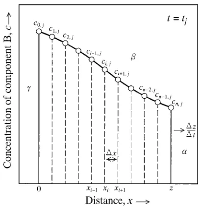
respectively. Here,iandjare the dimensionless integers that are equal to or greater than 0. The concentration profile of component B in thephase att¼tjis schematically shown

in Fig. 2. In this figure, the ordinate and the abscissa indicate the composition c and the distance x, respectively. Unlike Fig. 1, however, the distance x is measured from the = interface in Fig. 2. Hereafter, the origin of the distancexis defined in this manner. Furthermore,zis the position of the =interface measured from the origin of the distancex, and thus equivalent to the thickness of the phase. Thus, there exists the following relationship amongz,z andz.

z¼zz ð6Þ

In Fig. 2, the thickness zis divided into grid points with a number of nþ1. The interval xbetween the neighboring grid points is obtained by the relationshipx¼z=n. Hence,

z¼nx¼xn. The composition of the phase with x¼xi

andt¼tjis denoted byci;j. Sincezis a function oft,xalso

varies depending on t. In contrast, t is kept constant independently oft. The compositionsc0;jandcn;jcorrespond

to the values at the = and = interfaces, respectively. During annealing,ci;jchanges depending ontfor0<i<n,

but takes constant values ofc0;0orcandcn;0orcfori¼0 andn, respectively. Consequently, we obtain

rci1;jþ1þ2ð1þrÞci;jþ1rciþ1;jþ1

¼ ðrpivjÞci1;jþ2ð1rÞci;jþ ðrþpivjÞciþ1;j ð7aÞ

for1<i<n1,

2ð1þrÞc1;jþ1rc2;jþ1

¼ ð2rpivjÞc0;0þ2ð1rÞc1;jþ ðrþpivjÞc2;j ð7bÞ

fori¼1, and

rcn2;jþ1þ2ð1þrÞcn1;jþ1

¼ ðrpivjÞcn2;jþ2ð1rÞcn1;jþ ð2rþpivjÞcn;0 ð7cÞ fori¼n1. Here,randpiare defined as

r¼DðtjÞt

x2 ð8aÞ and

pi¼ it

2zjþ1

; ð8bÞ

respectively. The notation DðtjÞ explicitly indicates that D

varies depending on tj. The migration rate vj of the = interface measured from the = interface at t¼tj is obtained as

vj¼zj t ¼

zjþ1zj t ¼q

_ðc

2;j4c1;jþ3c0;0Þ

qðcn2;j4cn1;jþ3cn;0Þ; ð9Þ

whereqandq are defined as

q¼ DðtjÞ

2ðc_cÞx ð10aÞ and

q ¼ DðtjÞ

2ðc_cÞx; ð10bÞ

respectively. In eqs. (8b) and (9),zjandzjþ1are the positions of the = interface at t¼tj and tjþ1, respectively. Equation (7) is simply expressed using matrices A,B and Cas follows.

AC¼B ð11Þ

Here,

A¼

2ð1þrÞ r 0 . . . 0 0 r 2ð1þrÞ r . . . 0 0 0 r 2ð1þrÞ . . . 0 0

.. . .. . .. . . . . .. . .. .

0 0 0 r 2ð1þrÞ r

0 0 0 0 r 2ð1þrÞ 0 B B B B B B B B B @ 1 C C C C C C C C C A

; ð12aÞ

B¼

ð2rp1vjÞc0;0þ2ð1rÞc1;jþ ðrþp1vjÞc2;j

ðrp2vjÞc1;jþ2ð1rÞc2;jþ ðrþp2vjÞc3;j

ðrp3vjÞc2;jþ2ð1rÞc3;jþ ðrþp3vjÞc4;j

.. .

ðrpn2vjÞcn3;jþ2ð1rÞcn2;jþ ðrþpn2vjÞcn1;j

ðrpn1vjÞcn2;jþ2ð1rÞcn1;jþ ð2rþpn1vjÞcn;0 0 B B B B B B B B B B @ 1 C C C C C C C C C C A

ð12bÞ

and

C¼

c1;jþ1

c2;jþ1

c3;jþ1

.. .

cn2;jþ1

cn1;jþ1 0 B B B B B B B B B @ 1 C C C C C C C C C A

: ð12cÞ

The matrixCcomposed of the unknown compositionci;jþ1is calculated for the matrix Bcontaining the known composi-tion ci;j from eq. (11). Since the matrix Ais tridiagonal as

shown in eq. (12a), the calculation can be readily carried out by an appropriate linear algebra technique even for a large number ofn.50)

3. Results and Discussion

3.1 Growth behavior ofphase

In the present model, no diffusional flux exists in theand phases of the semi-infinite diffusion couple. In such a case, the growth of the phase is governed by the interdiffusion across the phase. Hence, the influence of grain growth on the kinetics of the mixed rate-controlling process is suitably emphasized in the present model. As mentioned earlier, the phase is formed as a layer in the semi-infinite diffusion couple. Hereafter, the layer of thephase is merely called the layer.

When the layer grows according to the mixed rate-controlling process and grain growth occurs in the layer, the diffusion coefficient D monotonically decreases with increasing annealing timetdue to the grain growth. In order

to express the diffusion coefficient DðtÞ as a mathematical function of the annealing timet, we assume that thelayer is composed of a single layer of square-rectangular grains with an identical dimension. Such a square-rectangular grain is schematically shown in Fig. 3. In this figure, d is the side length of the square basal-plane,zis the height, andis the thickness of the grain boundaries surrounding the grain. Here, the z axis is perpendicular to the interface, and hence the basal-plane is parallel to the interface. Consequently, the height of the square-rectangular grain is equivalent to the thickness of thelayer. On the other hand, the side lengthd

stands for the grain size of the square-rectangular grain. In this case, the fraction fof the total cross-sectional area for the grain boundaries to the whole cross-sectional area of the layer is evaluated by the following equation.

f ¼2

d ð13Þ

In order to simplify the analysis, the following assumptions were adopted for thelayer: (A) there is no grain boundary segregation; (B) volume and boundary diffusion takes place along the zaxis; and (C) grain growth starts to occur at a certain annealing time ofts. Due to assumptions A and B, the effective diffusion coefficientDacross thelayer is readily calculated by the equation

d¼dsþkd

td

t0

p

ð15Þ

Here,dsis the value of d attts,kd is the proportionality coefficient,pis the exponent,td¼tts, andt0is unit time, 1 s. The proportionality coefficient kd possesses the same dimension as d, but the exponent pis dimensionless. From eqs. (13)–(15),Dis finally expressed as an explicit function oft. Combining eqs. (13)–(15) with eqs. (8)–(12), the growth behavior of the layer was calculated numerically. In the present analysis, the following parameters were used for the whole numerical calculation: y¼0:1, y¼0:3, y¼ 0:7,y¼0:9,¼51010m andds¼106m. Here,yis the mol fraction of component B. Furthermore,tsis defined as the annealing time t where zreaches to ds. Hence, z<

d¼dsatt<ts, butz¼d¼dsatt¼ts. This means that the square-rectangular grain becomes the cubic grain with a side length ofds att¼ts. Att>ts, however, d becomes surely greater thands, but greater or smaller thanzdepending onkd andp. In Figs. 1 and 2, the composition is indicated with the concentration c of component B measured in mol per unit volume. On the other hand, the mol fractionyis practically used to express the composition of each phase. However, the mol fractionyis readily converted into the concentrationcby the equationc¼y=Vm, whereVmis the molar volume of the relevant phase. If the molar volume Vm is assumed to be constant independent of the composition, the concentration

ci;j in eqs. (9)–(12) is automatically replaced with the mol

fractionyi;j. Here, the subscriptsiandjof the mol fractiony

possess the same meanings as the concentration c. As previously mentioned, at tts, the grain growth does not occur and thusd¼ds. Therefore,Dis constant independent oftaccording to eqs. (13)–(15). In such a case,zjandyi;jare

calculated analytically.46,47) _{The analytical values ofz}

j and yi;jattj¼tswere used as the initial values for the numerical calculation of the new values attjþ1¼tjþt. The accuracy of the numerical calculation increases with decreasing values of x andt. However, very small values of x andt

result in an extremely long computing time. Thus, there is an optimum combination ofxandtdepending on the power of a computer. In the present analysis, a constant value of t¼0:1s was adopted for the numerical calculation up to

tjþ1¼107s. On the other hand, appropriate values ofnand x were determined from eq. (8a) and the equationx¼

z=nduring iteration in order to satisfyr<0:5.

Typical results for the numerical calculation are shown as

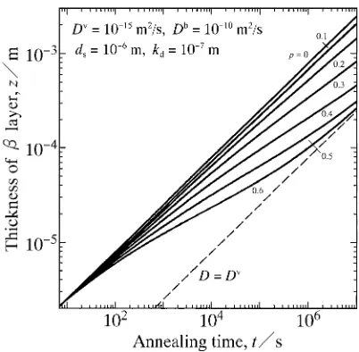
solid curves in Fig. 4. In this figure, the following parameters were used for the calculation:Dv_¼1015_m2_/s,Db _¼1010 m2_{/s, t}

s¼6:4s, kd¼107m and p¼0{0:6. In contrast, a dashed line indicates the result for the volume-diffusion controlling process with D¼Dv. In Fig. 4, the ordinate shows the logarithm of the thicknesszof thelayer, and the abscissa indicates the logarithm of the annealing timet. As can be seen, the thickness z monotonically increases with increasing annealing timet in different manners depending on the exponent p. For p¼0, the grain growth does not occur, and hence the fraction f remains constant during growth of thelayer. Therefore,Dis constant independent of

t. In such a case, the solid curve becomes straight, and hencez

is expressed as a power function oftby the equation

z¼k t t0

q

; ð16Þ

where k and q are the proportionality coefficient and the exponent, respectively. For the straight solid line withp¼0 in Fig. 4,k¼7:88107m andq¼0:5are obtained from eq. (16). On the other hand, the dashed line provides k¼ 7:84108m andq¼0:5. Thus, the parabolic relationship holds good not only for the volume-diffusion controlling process but also for the mixed rate-controlling process without grain growth. However,kis one order of magnitude greater for the latter rate-controlling process than for the former rate-controlling process. Thus, the growth of the layer is accelerated by the boundary diffusion, though the parabolic relationship holds good in both rate-controlling processes.

Sinced¼dsattts, the solid curves for p>0coincide with the solid line for p¼0attts. As the annealing timet

increases at t>ts, however, the solid curves gradually deviate from the solid line, and then asymptotically approach to the dashed line. The rate of the approach to the dashed line increases with increasing value ofpat a constant value ofkd. For such solid curves, z cannot be expressed as a power function oftwith a constant value ofq. The dependence ofq

ontwas evaluated from the following equation usingzjand Fig. 4 The thicknesszof thelayer versus the annealing timetcalculated

forDv_¼1015_m2_/s,Db_¼1010_m2_/s,k

d¼107m and p¼0{0:6. A dashed line shows the calculation forD¼Dv_.

zjþ1 att¼tjandtjþ1, respectively.

q¼lnðzjþ1=zjÞ

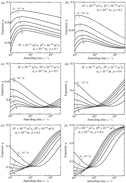
lnðtjþ1=tjÞ ð17Þ The evaluation was carried out for the solid curves in Fig. 4. The results for p¼0:1{0:6 are shown as solid curves in Fig. 5(a)–(f), respectively. The evaluation was executed further for kd¼2107{6107m as well as kd¼1 107_{m. The corresponding results for p¼0:1{0:6are also} indicated as solid curves in Fig. 5(a)–(f), respectively. In this figure, the ordinate shows q, and the abscissa indicates the logarithm oft. Forp¼0:1in Fig. 5(a),qattains to maximum values at annealing times around t¼103s. In contrast, q

monotonically decreases with increasing value ofkd. Never-theless,qis rather close to 0.5 att¼102{107s. Although a similar tendency is recognized also forp¼0:2in Fig. 5(b),q

is slightly smaller for p¼0:2than forp¼0:1. On the other hand, for p¼0:3 in Fig. 5(c), q varies depending on t in complicated manners. Nonetheless, q reaches to an almost constant plateau value of qc¼0:38 at a certain annealing time oft¼tc. Here, the term ‘‘plateau’’ means thatqis rather insensitive to t at annealing times around t¼tc. Thus, eq. (16) approximately holds good at the plateau stage. The critical annealing time tc for the plateau value q¼qc monotonically decreases with increasing value of kd. Ac-cording to the results in Fig. 5(d)–(f), qc¼0:34, 0.30 and 0.27 for p¼0:4, 0.5 and 0.6, respectively. Furthermore, the solid curve forkd¼6107m in Fig. 5(b) givesqc¼0:42 for p¼0:2, and the solid line in Fig. 4 providesqc¼0:5for

p¼0. These values ofqcare plotted as open circles against the exponent pin Fig. 6. As can be seen,qcmonotonically decreases from 0.5 to 0.27 with increasing value of pfrom 0 to 0.6. Consequently, the exponentqcbecomes much smaller than 0.5 on condition that the grain growth occurs consid-erably in thelayer. A solid curve passing through the open circles is slightly convex downwards at p>0:4, but almost straight atp<0:4. Thus, there exists an approximately linear relationship betweenqcandpat p<0:4.

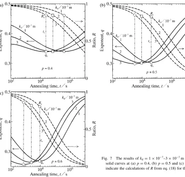
The results for p¼0:4{0:6 in Fig. 5(d)–(f) are shown again as solid curves in Fig. 7(a)–(c), respectively. However, only the results of kd¼1107{3107m indicating rather clear plateau stages are represented in Fig. 7. In this figure, the ordinate on the left-hand side indicatesq, and the abscissa shows the logarithm oft. As the annealing timet

increases,qgradually decreases att<tc, and then reaches to

qc at t¼tc. On the other hand, at t>tc,q monotonically increases with increasing annealing timet. Unlike Fig. 5(c)– (f), however, tc is longer than 107s for most of the solid curves in Fig. 5(a) and (b). Hence,qccannot appear on these solid curves. Such annealing time dependence of q is attributed to variation in the contribution of the boundary diffusion to the effective diffusion in thelayer. In order to examine such variation, the ratioRis defined as

R¼ fD b

D : ð18Þ

From eq. (18),Rwas calculated as a function oft. The results for the solid curves are shown as dashed curves in Fig. 7. In this figure, the ordinate on the right-hand side indicates R. Furthermore, Rc andqc are shown as open circles, squares

and rhombuses forkd¼1107,2107and3107m, respectively. Here,Rcstands for the value ofRatt¼tc. As can be seen, R monotonically decreases with increasing annealing time t. This means that the contribution of the boundary diffusion gradually decreases due to the grain growth in thelayer.

The values of Rc for kd¼1107, 2107 and 3 107_{m in Fig. 7 are plotted as open circles, squares and} rhombuses, respectively, against the exponentpin Fig. 8. As can be seen, Rc is close to 0.85 at p¼0:4 for kd¼1 107{3107m, and remains almost constant independ-ently of pforkd¼3107m. However, forkd¼1107 and2107m,Rcslightly decreases with increasing value of p. Even in such a case, Rc is still greater than 0.8 at

p¼0:6. This means that the contribution of the boundary diffusion is more than 80 percent at t¼tc. As shown in Fig. 7, the exponent q starts to increase with increasing annealing time att¼tc. However, att¼tc, the contribution of the volume diffusion is less than 20 percent. Consequently, the growth of the layer is predominantly governed by the boundary diffusion at the plateau stage withq¼qc.

The dependence of the exponent q on the ratio R was estimated from the solid and dashed curves in Fig. 7. The results ofkd¼1107,2107 and3107m are shown as solid curves interconnecting open circles, squares and rhombuses, respectively, in Fig. 9. In this figure, the open symbols on the right-hand side showRcandqcatt¼tc, and those on the left-hand side indicateRandq att¼107s. As can be seen,Rc takes values between 0.80 and 0.85. As the annealing time increases fromt¼tctot¼ 1s, the ratio will decrease from R¼Rc to R¼0, but the exponent should increase fromq¼qctoq¼0:5. The dependence ofqonR considerably varies depending on p, but the solid curves for different values of kd almost coincide with one another for each value of p. Therefore, the dependence of q on R is predominantly determined by p but not by kd, though the kinetics of the grain growth is controlled by bothkd and p. The corresponding calculation was carried out also forDv_¼ 1016_m2_{/s andD}b_¼1011_m2_{/s at p¼0:5. Here, the ratio}

Dv_=Db _{is the same as D}v_¼1015_m2_{/s and D}b _¼1010 m2/s. The results with kd¼1107 and 3107m are shown as solid curves interconnecting open triangles and inverse-triangles, respectively, in Fig. 9. As can be seen, the solid curves with the open triangles and inverse-triangles coincide well with those with the open circles, squares and rhombuses for p¼0:5. This means that the dependence ofq

onRis insensitive to the values ofDv _andDb _{as long as the} ratioDv_=Db_{is identical.}

The semblable calculation was carried out for various values of Dv _{at D}b_¼1010_m2_{/s, k}

d¼3107m and

p¼0:5. The results forDv_¼1015_,1016 _and1017_m2_/s are shown as solid curves interconnecting open circles, squares and rhombuses, respectively, in Fig. 10. Also in this figure, the open symbols on the right-hand side indicateRc andqcatt¼tc, and those on the left-hand side showRandq att¼107s. AsDvdecreases from1015m2/s to1017m2/s,

annealing time where the contribution of the volume diffusion is merely 3 percent. Considering the curvature, we may expect that the solid curves coincide well with one another at small values of R. As a result, it is concluded that the dependence of q on R varies depending on Dv at large values of R but becomes insensitive to Dv at small values ofR.

3.2 Comparison with previous analyses

As mentioned in Sect. 1, the kinetics of the mixed rate-controlling process was theoretically analyzed by Farrell and Glimer.34)Like the present analysis, they considered a semi-infinite diffusion couple initially consisting of two solid-solution phases with solubility compositions. Thus, there is no diffusional flux in both solid-solution phases. In such a Fig. 5 The exponentqversus the annealing timetcalculated forDv_¼1015_m2_/s,Db_¼1010_m2_{/s andk}

semi-infinite diffusion couple, a polycrystalline compound layer is formed at the interface between the solid-solution phases. Here, the compound layer with a thickness of z is composed of flat grain boundaries with a thickness ofand tabular grains, and each tabular grain is sandwiched between two parallel grain boundaries perpendicular to the interface. The distance d between the neighboring parallel grain

boundaries is identical for all the tabular grains, and the d

axis and thezaxis are perpendicular to the grain boundary and the interface, respectively. For such a compound layer, the one-dimensional boundary diffusion along thezaxis and the two-dimensional volume diffusion along the d axis and the z axis were calculated numerically. Unlike the present analysis, however, the grain size d remains constant during Fig. 8 The ratioRcatt¼tcversus the exponentpfor the results in Fig. 7 with kd¼1107, 2107 and 3107m shown as open circles, squares and rhombuses, respectively.

Fig. 6 The exponentqcversus the exponentpforDv¼1015m2/s and Db_¼1010_m2_{/s shown as open circles. Open squares indicate the values} smaller by 8 percent thanqc, and a dotted line shows the result deduced from the mathematical model of Corcoranet al.35)

growth of the compound layer. This corresponds to the growth with p¼0. Their analysis indicates that z is expressed as a power function oftby eq. (16) andqis equal to 0.48. In contrast, the present analysis gives q¼0:5 for

p¼0as shown in Fig. 4. The discrepancy betweenq¼0:48 and 0.5 is attributed to the volume diffusion along thedaxis. In order for the compound layer to grow continuously, solute atoms should be transported by the boundary diffusion along the grain boundary parallel to thezaxis over long distances. However, the solute atoms in the grain boundary may be partially wasted by the volume diffusion along the d axis. Such wastage will decelerate the growth of the compound layer. Also in the present analysis, it is possible to consider

the volume diffusion along the d axis. However, in the square-rectangular grain, there are doubled-axes perpendic-ular to each other. In such a case, the two-dimensional volume diffusion along the doubled-axes as well as the one-dimensional volume diffusion along the z axis has to be calculated numerically. However, an unrealistically long computing time is necessary for such a three-dimensional numerical calculation. Consequently, in the present analysis, the one-dimensional volume diffusion along the zaxis was considered, but the two-dimensional volume diffusion along the doubled-axes was omitted. Nevertheless, influence of the omission on the kinetics can be estimated from the analysis of Farrell and Glimer.34) According to their analysis, q is decreased by 4 percent due to the one-dimensional volume diffusion along the single d axis. Consequently, q may be diminished by 8 percent owing to the tow-dimensional volume diffusion along the double d-axes. In Fig. 6, open squares show the values ofqcsmaller by 8 percent than those with the open circles. In the present analysis, however, the grain sizedmonotonically increases with increasing anneal-ing time at t>ts. The penetration depth of the volume diffusion along thedaxis relative to the grain sizedis smaller for the growing grain than for the non-growing grain. Hence, the diminishment may be smaller than 8 percent at large values of p. Consequently, the open squares provide the lower limit for the estimation ofqc.

On the other hand, as mentioned in Sect. 1, the growth of a compound layer controlled by boundary diffusion was theoretically analyzed by Corcoranet al.35)In their analysis, a compound layer in a semi-infinite diffusion couple consists of cylindrical grains with an identical diameter ofd, where the rotation axis of the grain with a length of z is perpendicular to the interface and the diameter d increases in proportion to a power function of the annealing timetwith an exponent ofp. Thus, the thickness of the compound layer is equal toz. Furthermore, only boundary diffusion occurs in the compound layer, but volume diffusion takes place merely in the neighboring phase ahead of the growing compound layer. If the boundary diffusion predominantly governs the growth of the compound layer, the thicknesszis expressed as a power function of the annealing timetwith an exponent of

q. In such a case, the following relationship holds good between pandq.35)

q¼1p

2 ð19Þ

The relationship of eq. (19) is shown as a dotted line in Fig. 6. As can be seen, the slope is steeper for the dotted line than for the dashed and solid curves passing through the open squares and circles, respectively. Nevertheless, at p¼0:2{ 0:4,qis rather close to each other between the dashed curve and the dotted line. Consequently, the relationship betweenp

and q is approximately described by eq. (19) in the range of p¼0:2{0:4, even though the two-dimensional volume diffusion along the doubled-axes is omitted in eq. (19).

4. Conclusions

The kinetics of the reactive diffusion controlled by boundary and volume diffusion was numerically analyzed Fig. 9 The exponentqversus the ratioRat annealing times betweent¼tc

and 107_{s for the results in Fig. 7 with k}

d¼1107, 2107 and 3107_{m shown as solid curves interconnecting open circles, squares} and rhombuses, respectively. The results for Dv_¼1016_m2_/s,

Db_¼1011_m2_{/s, p¼0:5 and k}

d¼1107 and 3107m are indicated as solid curves interconnecting open triangles and inverse-triangles, respectively.

for a hypothetical binary system consisting of one interme-tallic compound and two primary solid-solution phases using a mathematical model of a semi-infinite diffusion couple. Here, the diffusion couple is initially composed of the two primary solid-solution phases with solubility compositions. During isothermal annealing at a certain temperature, a layer of the intermetallic compound is formed at the interface in the diffusion couple due to the reactive diffusion between the primary solid-solution phases. However, there is no diffu-sional flux in the primary solid-solution phases. On the other hand, the compound layer consists of a single layer of square-rectangular grains with an identical dimension, where the side length of the basal-plane and the height are d and z, respectively. Thezaxis is perpendicular to the interface, and hence the basal-plane is parallel to the interface. Therefore, the thickness of the compound layer is equal to z. For simplification of the analysis, the following assumptions were adopted for the compound layer: (A) there is no grain boundary segregation; (B) volume and boundary diffusion occurs along thezaxis; and (C) grain growth starts to occur at a certain annealing time. In order to calculate numerically the growth rate of the compound layer, Crank-Nicolson implicit method48)_{was combined with a finite-difference technique.}49) When the grain sizedremains constant during growth of the compound layer, the thickness of the compound layer is proportional to a power function of the annealing timetand the exponent q of the power function is equal to 0.5. In contrast,qvaries depending ontin complicated manners, ifd

increases in proportion to a power function oft. Around the critical annealing timetc, however,qis rather insensitive tot. A constant value of q at t¼tc is denoted by qc. If the diffusion coefficient is five orders of magnitude greater for the boundary diffusion than for the volume diffusion,qctakes values of 0.5, 0.42, 0.38, 0.34, 0.30 and 0.27 at p¼0, 0.2, 0.3, 0.4, 0.5 and 0.6, respectively. Here, pis the exponent of the power function for the grain growth. Considering the influence of the two-dimensional volume diffusion perpen-dicular to the grain boundary on the kinetics, we obtain

qc¼0:46, 0.39, 0.35, 0.32, 0.28 and 0.25 atp¼0, 0.2, 0.3, 0.4, 0.5 and 0.6, respectively. Consequently, atp¼0:2{0:4,

qc is approximately expressed as a function of p by the equation qc¼ ð1pÞ=2 deduced from the mathematical model of Corcoranet al.35)

Acknowledgement

The present study was supported by the Iketani Science and Technology Foundation in Japan.

REFERENCES

1) B. Lustman and R. F. Mehl: Trans. Met. Soc. AIME147(1942) 369– 394.

2) D. Horstmann: Stahl. Eisen.73(1953) 659–665.

3) S. Storchheim, J. L. Zambrow and H. H. Hausner: Trans. Met. Soc. AIME200(1954) 269–274.

4) L. S. Castleman and L. L. Seigle: Trans. Met. Soc. AIME209(1957) 1173–1174.

5) L. S. Castleman and L. L. Seigle: Trans. Met. Soc. AIME212(1958)

589–596.

6) N. L. Peterson and R. E. Ogilvie: Trans. Met. Soc. AIME218(1960) 439–443.

7) Y. Adda, M. Beyeler, A. Kirianenko and M. F. Mauruce: Mem. Sci. Rev. Met.58(1961) 716–724.

8) L. S. Birks and R. E. Seebold: J. Nucl. Mater.3(1961) 249–259. 9) R. E. Seebold and L. S. Birks: J. Nucl. Mater.3(1961) 260–266. 10) G. V. Kidson and G. D. Miller: J. Nucl. Mater.12(1964) 61–69. 11) W. E. Sweeney, Jr. and A. P. Batt: J. Nucl. Mater.13(1964) 87–91. 12) K. Shibata, S. Morozumi and S. Koda: J. Japan Inst. Met.30(1966)

382–388.

13) K. Hirano and Y. Ipposhi: J. Japan Inst. Met.32(1968) 815–821. 14) T. Nishizawa and A. Chiba: J. Japan Inst. Met.34(1970) 629–637. 15) M. M. P. Janssen: Metall. Trans.4(1973) 1623–1633.

16) G. F. Bastin and G. D. Rieck: Metall. Trans.5(1974) 1817–1826. 17) M. Onishi and H. Fujibuchi: Trans. JIM16(1975) 539–547. 18) E. I.-B. Hannech and C. R. Hall: Mater. Sci. Tech.8(1992) 817–824. 19) P. T. Vianco, P. F. Hlava and A. L. Kilgo: J. Electron. Mater.23(1994)

583–594.

20) M. Watanabe, Z. Horita and M. Nemoto: Interface Science4(1997) 229–241.

21) S. Choi, T. R. Bieler, J. P. Lucas and K. N. Subramanian: J. Electron. Mater.28(1999) 1209–1215.

22) T. Takenaka, M. Kajihara, N. Kurokawa and K. Sakamoto: Mater. Sci. Eng. A406(2005) 134–141.

23) Y. Muranishi and M. Kajihara: Mater. Sci. Eng. A404(2005) 33–41. 24) T. Hayase and M. Kajihara: Mater. Sci. Eng. A433(2006) 83–89. 25) Y. Tanaka, M. Kajihara and Y. Watanabe: Mater. Sci. Eng. A445–446

(2007) 355–363.

26) D. Naoi and M. Kajihara: Mater. Sci. Eng. A459(2007) 375–382. 27) K. Mikami and M. Kajihara: J. Mater. Sci.42(2007) 8178–8188. 28) M. Kajihara, T. Yamada, K. Miura, N. Kurokawa and K. Sakamoto:

Netsushori43(2003) 297–298.

29) T. Yamada, K. Miura, M. Kajihara, N. Kurokawa and K. Sakamoto: J. Mater. Sci.39(2004) 2327–2334.

30) T. Yamada, K. Miura, M. Kajihara, N. Kurokawa and K. Sakamoto: Mater. Sci. Eng. A390(2005) 118–126.

31) M. Kajihara and T. Takenaka: Mater. Sci. Forum 539–543(2007) 2473–2478.

32) J. D. Baird: J. Nucl. Energy A11(1960) 81–88.

33) F. Brossa, A. Hubaux, D. Quataert and H. W. Schleicher: Mem. Sci. Rev. Metall.63(1966) 1–10.

34) H. H. Farrell and G. H. Glimer: J. Appl. Phys.45(1974) 4025–4035. 35) Y. L. Corcoran, A. H. King, N. de Lanerolle and B. Kim: J. Electron.

Mater.19(1990) 1177–1183.

36) K. Suzuki, S. Kano, M. Kajihara, N. Kurokawa and K. Sakamoto: Mater. Trans.46(2005) 969–973.

37) M. Mita, M. Kajihara, N. Kurokawa and K. Sakamoto: Mater. Sci. Eng. A403(2005) 269–275.

38) T. Takenaka, S. Kano, M. Kajihara, N. Kurokawa and K. Sakamoto: Mater. Sci. Eng. A396(2005) 115–123.

39) T. Takenaka, S. Kano, M. Kajihara, N. Kurokawa and K. Sakamoto: Mater. Trans.46(2005) 1825–1832.

40) M. Mita, K. Miura, T. Takenaka, M. Kajihara, N. Kurokawa and K. Sakamoto: Mater. Sci. Eng. B126(2006) 37–43.

41) T. Takenaka and M. Kajihara: Mater. Trans.47(2006) 822–828. 42) T. Takenaka, M. Kajihara, N. Kurokawa and K. Sakamoto: Mater. Sci.

Eng. A427(2006) 210–222.

43) Y. Yato and M. Kajihara: Mater. Sci. Eng. A428(2006) 276–283. 44) Y. Yato and M. Kajihara: Mater. Trans.47(2006) 2277–2284. 45) S. Sasaki and M. Kajihara: Mater. Trans.48(2007) 2642–2649. 46) W. Jost: Diffusion of Solids, Liquids, Gases (Academic Press, New

York, 1960) p. 68.

47) M. Kajihara: Acta Mater.52(2004) 1193–1200.

48) J. Crank: The Mathematics of Diffusion (Oxford Univ. Press, London, 1979) p. 144.

49) R. A. Tanzilli and R. W. Heckel: Trans. Met. Soc. AIME242(1968) 2313–2321.