Bayesian Inference in Spatial Sample Selection Models

Munich Personal RePEc Archive

Bayesian Inference in Spatial Sample

Selection Models

Dogan, Osman and Taspinar, Suleyman

16 December 2016

Online at

https://mpra.ub.uni-muenchen.de/82829/

Bayesian Inference in Spatial Sample Selection Models

Osman Do˘gan† S¨uleyman Ta¸spınar‡

December16, 2016

Abstract

In this study, we consider Bayesian methods for the estimation of a sample selection model with spatially correlated disturbance terms. We design a set of Markov chain Monte Carlo (MCMC) algorithms based on the method of data augmentation. The natural parameterization for the covariance structure of our model involves an unidentified parameter that complicates posterior analysis. The unidentified parameter – the variance of the disturbance term in the selection equation – is handled in different ways in these algorithms to achieve identification for other parameters. The Bayesian estimator based on these algorithms can account for the selection bias and the full covariance structure implied by the spatial correlation. We illustrate the implementation of these algorithms through a simulation study.

JEL-Classification: C13, C21, C31

Keywords: Spatial dependence, Spatial sample selection model, Bayesian analysis, Data augmen-tation.

∗_{This research was supported, in part, by a grant of computer time from the City University of New York High}

Performance Computing Center under NSF Grants CNS-0855217, CNS-0958379 and ACI-1126113.

†_{Project Department, Metro Istanbul, Esenler, Istanbul, Turkey, email: [email protected].}

‡_{Economics Program, Queens College, The City University of New York, New York, United States, email:}

1

Introduction

A typical sample selection model consists of (i) a selection equation that models the selection mech-anism through which we observe the level of outcome, and (ii) an outcome equation that describes the process that is generating the outcome. The model structure is characterized by the correlation between the disturbances of these equations, for which estimation requires special methods (Heck-man, 1979, 1990; Lee, 1978, 1994; Newey, 2009; Olsen, 1980). Besides the cross equation correlation in the disturbance terms, spatial correlation may also be present in the disturbance terms of each equation. The spatial sample selection model considered in the present study accommodates both type of correlations.

Selection models, or more generally Type-I or Type-II type Tobit models, may arise frequently in urban economics, regional science, labor economics, agricultural economics, and social interaction models. It is natural to consider a notion of spatial correlation in the unobservables so long as data is organized by a notion of location in the relevant space. The presence of common shocks, factors, cluster effects provides a natural motivation. For example, McMillen, (1995) studies residential land values in urban areas through a sample selection model. He conjectures that unobserved variables that make a parcel more likely to receive residential zoning may increase the value of residential land. It is also plausible to allow for spatially correlated disturbance terms because nearby parcels are likely to be affected by the same neighborhood factors and spillovers. B¨uchel and Ham, (2003) studies overeducation– a job seeker’s overqualification for a job she accepts due to her location constraints– through a Heckit model. The selection problem arises because overeducation observed only for the employed. The authors state that the risk of overeducation largely determined by spatial flexibility of a job seeker in combination with the spatial heterogeneity in suitable job opportunities, relative to the place of residence. They try to control for spatial correlations in the disturbance terms by clustering methods. Flores-Lagunes and Schnier, (2012) study (for details, see our empirical illustration) the spatial production of fisheries in the Eastern Bering Sea through a sample selection model. Since a negative shock that affects the fish population in a certain location would affect the production of all vessels in other locations by displacing fishing effort into more efficient surrounding locations, they allow disturbance terms to be spatially correlated.

Another motivation for considering spatial correlation is related to measurement error. The mismatch between the spatial unit of observations (e.g., census tract, county, state, peer groups, farm location, fishing zone etc.) and the unit of a study (e.g., student, household, housing market, labor market, farm, fishing vessel, etc.) can cause measurement errors in the variables of interest (Anselin, 2007). Since these measurement errors may vary systematically across space, the distur-bance terms of a regression model over the same space are likely to be correlated. Ward et al., (2014) consider a sample selection model of cereal production where the selection equation specifies a farmer’s endogenous decision about whether to plant cereals. They employ a first-order spatial autoregressive model for the disturbance terms, because data on yields or climate are aggregated for large administrative units, and correlation among unobservables may be driven by unobserved en-vironmental, geographical and climatological clusters. Raboviˇc and ˇC´ıˇzek, (2016) provides another example in the context of peer effects, where the outcome equation models a student’s achievement on a test and the selection equation models the student’s decision whether to take the exam. It is plausible that decision to take the exam and the score from the exam may depend on a student’s ability that is likely to be similar to her peers’ abilities. Therefore, social interaction literature often incorporate what is known as the “correlated effects” in the model (Lee et al., 2010).

distribution function, which often leads to numerical estimation problems. To circumvent this shortcoming of the MLE, alternative methods have been suggested in the literature. For example, McMillen, (1992) uses an expectation maximization (EM) algorithm to circumvent the evaluation of the multivariate normal distribution function and suggests a tractable iterative estimation approach. Beron and Vijverberg, (2004) use the recursive importance sampling (RIS) simulator to approximate the log-likelihood function of the spatial probit model. Pinkse and Slade, (1998) formulate moment functions from the score vector of a partial MLE for the generalized method of moments (GMM) estimation of a spatial probit model. Instead of using entire joint distribution of observations implied by the spatial dependence, Wang et al., (2013) formulate a partial MLE based on the partial joint distribution of observations to reduce computational difficulties.

McMillen, (1995) extends the EM algorithm suggested in McMillen, (1992) to a sample selection model that has a first order spatial autoregressive process in the disturbance term. The estimation scheme requires inversion of ann_×nmatrix at each iteration which makes this approach impractical for large samples. Flores-Lagunes and Schnier, (2012) combine the GMM approach in Pinkse and Slade, (1998) and Kelejian and Prucha, (1998) and suggest a GMM method for a sample selection model that has a first order spatial autoregressive process in the disturbance terms. The moment functions for the estimation of the selection equation are the ones suggested by Pinkse and Slade, (1998) for the probit model. These moment functions are combined with the moment functions formulated for the outcome equation to form a joint GMME. The simulation studies reported in Flores-Lagunes and Schnier, (2012) show that the bias present in the selection equation parameters adversely affects the estimation of the parameter of the outcome equation. Raboviˇc and ˇC´ıˇzek, (2016) extends the partial maximum likelihood (ML) method of Wang et al., (2013) to a sample selection model with a spatial lag of a latent dependent variable and a sample selection model with spatially correlated disturbance terms. They establish the large sample properties of the proposed partial MLE and provide a finite sample bias and precision comparison to the Heckit and the GMM approach of Flores-Lagunes and Schnier, (2012). Overall, the proposed partial MLE outperforms the Heckit and the GMM based estimator.

In this paper, we consider a sample selection model that has a first order spatial autoregres-sive process for the disturbance terms of the selection and outcome equations.1 _{We consider the}

Bayesian MCMC estimation approach for this model with various alternative Gibbs samplers. In comparison with the GMM and partial ML approaches, the Bayesian approach with data augmenta-tion formulates estimators that can exploit the full informaaugmenta-tion on the spatial correlaaugmenta-tion structure. The data augmentation method treats the underlying latent variable as an additional parameter to be estimated and this treatment of latent variables facilitates the posterior simulation through an MCMC sampler (Albert and Chib, 1993; van Dyk and Meng, 2001). The natural parameterization for the covariance of our model involves an unidentified parameter which can complicate posterior analysis. The unidentified parameter, i.e., the variance of the disturbance terms in the selection equation, is handled in different ways in the suggested Gibbs samplers.

In the first algorithm, we specify prior distributions for the identified parameters and consider the method suggested in Nobile, (2000) that can be used to construct a Markov chain that fixes the unidentified parameter during the posterior analysis. In the second algorithm, we consider the re-parameterization approach suggested in Li, (1998), McCulloch et al., (2000) and van Hasselt, (2011) for the covariance matrix of the model. Given the bivariate normal distribution assumption for the disturbance terms, the covariance matrix is re-parameterized in terms of conditional variance and covariance of disturbance terms. In the third algorithm, we consider a different blocking scheme for

1

the full set of conditional posterior distributions. The Gibbs sampler operates by splitting the full set of parameters into different blocks which can affect the mixing properties of the sampler. Hence, we consider an alternative sampler where the parameter vector of the regressors in the outcome equation and covariance term of the disturbance terms are sampled through a single block.

In the fourth and fifth algorithms, we consider samplers based on the parameter expansion method (or the marginal data augmentation method) for the estimation of our model (Liu and Wu, 1999; Meng and van Dyk, 1999). The unidentified parameter, i.e., the variance of the disturbance term in the selection equation, is introduced in the sampler through an appropriate prior distribution to improve the convergence properties of the sampler. The proper prior distributions that can be assigned to the unidentified parameter do not affect the posterior distribution of the identified model parameters in these samplers but can improve the characteristics of the resulting Markov chains. As a result, these algorithms accommodate the normalization constraint in the estimation while improving the convergence rates of the resulting Markov chains.

Through a simulation study, we illustrate the implementation of these algorithms in the context of our spatial sample selection model. Our results show that the Bayesian estimator in all algorithms reports estimates that are close to the true parameter value for the autoregressive parameter of the selection equation. For the autoregressive parameter in the outcome equation, the deviation of the posterior mean estimate from the true parameter value is negligible for the Bayesian estimator in Algorithms 1–4. As for the parameters of the exogenous variables in the selection and outcome equations, the Bayesian estimator in Algorithms 1 and 4 performs relatively better in terms of reported deviations between the point estimates and the true parameter values. Our results also indicate that all algorithms have similar mixing properties under our priors specifications. For an empirical illustration, we use the application in the area of natural resource economics considered in Flores-Lagunes and Schnier, (2012) to model the spatial production within a fishery with a spatial sample selection model. Our Bayesian estimator reports much precise estimates for this application as it accounts for the full covariance structure implied by the spatial correlation.

The remainder of this article is divided into five sections. In Section 2, we provide the model specification. In Section 3, we provide the posterior analysis including prior specifications. We present the details of our simulation design in Section 4. We evaluate the relative performance of algorithms in this section. In Section 5, we provide an empirical illustration and examine the relevance of Bayesian estimates in comparison with the estimates from a GMME suggested by Flores-Lagunes and Schnier, (2012). Section 6 concludes. Some technical results and figures are left to a web appendix.

2

Model Specification

We consider the following Type II Tobit model with a first order spatial autoregressive process:

Y₁⋆_i=X₁′_iβ+U1i, U1i=λ n X

j=1

WijU1j+ε1i, (2.1)

Y₂⋆_i=X₂′_iδ+U2i, U2i =ρ n X

j=1

MijU2j+ε2i, (2.2)

for i= 1, . . . , n. Here, Y₁⋆_i and Y₂⋆_i are, respectively, the latent variables of selection and outcome equations, X1i and X2i are, respectively, k1 ×1 and k2 ×1 vectors of non-stochastic exogenous

matrices of known constants with zero diagonal elements. The (i, j)th element of these matrices are respectively denoted byWij andMij in (2.1) and (2.2). Hence, the regression disturbance term

U1i andU2i are allowed to depend on the disturbance terms of other observations. The parameters

λandρ are known as the spatial autoregressive parameters. The innovations termsε1i and ε2i are

assumed to be i.i.dN(0,Σ) with

Σ =

σ₁2= 1 σ12

σ12 σ22

=

1 ̺σ2

̺σ2 σ22

(2.3)

where̺is the correlation coefficient betweenε1i andε2i. The observed variableY1i for the selection

equation is related to the latent variable Y₁⋆_i by Y1i =I(Y1⋆i >0) for i= 1, . . . , n, where I(·) is the

indicator function. The observed variableY2i for the outcome equation is related to both the latent

variables of the selection and outcome equations by

Y2i= (

Y₂⋆_i=X₂′_iδ+U2i if Y1i = 1

missing if Y1i = 0

(2.4)

for i = 1, . . . , n. For the non-spatial model where λ = ρ = 0, the OLS estimator of δ based on the subsample obtained when Y1i = 1 is inconsistent when σ12 6= 0. This result is the well-known

selectivity bias problem (Heckman, 1979).2

There are two identification issues related to sample selection models: (i) the normalization imposed on the variance of ε1i, and (ii) the exclusion restriction. Without the normalization

σ₁2 = 1, multiple values for the model parameters give rise to the same value for the likelihood function. Hence, the normalization can be considered as a way to achieve identification. The exclusion restriction, on the other hand, is relevant for the precision of estimator rather than for the identification of parameters. When there is no exclusion restriction, i.e., X1i = X2i, the

parameters are still identified within the ML framework (Lee, 2003; Wooldridge, 2002).3 However, if an excluded variable from the outcome equation is a relevant variable, i.e., when the exclusion restriction is false, then the suggested estimator will suffer from the omitted variable bias (Lee, 2003).4

For the Bayesian estimation of non-spatial sample selection model, the data is usually stacked for each pair of the latent observations such that theith observation is a vector denoted by Y⋆

i =

(Y₁⋆_i, Y₂⋆_i)′. Hence, the model can be written in a compact way by stacking over the pair of the

2

In the literature, there are other variants of the non-spatial sample selection model. For example, van Hasselt, (2005) and Wooldridge, (2002) suggest a two-part model where the outcome equation is different than that of the Type II Tobit model. The difference arises because the two-part model assumes that the disturbance termsU1i and

U2i are independent conditional on Y1⋆i > 0. Another closely related variant is the Roy Model (or Type V Tobit

model) which is a three equation model, where the first equation determines a selection outcome and the remaining two equations describe the main outcome for the cases ofY1i = 1 andY1i= 0, respectively. Li, (1998) considers a

variant in which the outcome equation is a Tobit equation. Hence, the observed variable for the outcome equation does not depend on the observed variable of the selection equation. In the variant considered by Chib et al., (2009), the selection equation is a Tobit type equation, and the observed variable of the outcome equation depends on the observed variable of the selection equation.

3_{There is also no identification problem for the Heckit of Heckman, (1979). However, this situation can introduce}

severe collinearity betweenX2iand the inverse Mills ratio, which can lead to imprecise estimators. The ML estimator

may also show poor performance when there is no exclusion restriction. For some simulation evidence, see Leung and Yu, (1996).

4

latent observations. Due to the presence of spatial dependence in disturbance terms, we do not use the same format for our model. Instead, we stack each equation independently and get

Y₁⋆ =X1β+S−1(λ)ε1, Y2⋆ =X2δ+R−1(ρ)ε2, (2.5)

where S(λ) = (In−λW), R(ρ) = (In−ρM), Yj⋆ = (Yj⋆1, Yj⋆2, . . . , Yjn⋆)

′

, Xj = (X

′

j1, X

′

j2, . . . , X

′

jn)

′

and εj = (εj1, εj2, . . . , εjn)

′

for j = 1,2. Let θ = (β′, δ′)′ be the augmented parameter vector.

Furthermore, let Y⋆ = Y₁⋆′, Y₂⋆′′

, X =

X1 0n×k2

0n×k1 X2

and ε= ε′₁S−1′(λ), ε′₂R−1′(ρ)′

. Then,

our model can be more compactly written as

Y⋆ =Xθ+ε, and E(εε′) = Ω =_K(λ, ρ) Σ_⊗InK

′

(λ, ρ), (2.6)

where_K(λ, ρ) =

S−1(λ) 0n×n

0n×n R−1(ρ)

.

3

Posterior Analysis

For the posterior analysis, the prior distributions need to be assigned to parameters of the model. We assume that the prior distribution functions of parameters of the model are independent. Let p(θ, λ, ρ,Σ) =p(θ)p(λ)p(ρ)p(Σ) be the joint prior distribution function. We assume the following prior distribution functions:

p(θ) = (2π)−k/2_|V0|−1/2exp

−1

2(θ−µ0)

′

V₀−1(θ₋µ0)

, (3.1)

p(Σ) =

2v0_π1/2

2

Y

i=1

Γ v0+ 1−i 2

−1

|T0|v0/2|Σ|−(v0+3)/2exp

− 1

2tr T0Σ

−1

I(Σ11= 1),

(3.2)

p(λ) =

(

κ1/2 ifλ∈(−1/κ1,1/κ1)

0 otherwise , (3.3)

p(ρ) =

(

κ2/2 ifρ∈(−1/κ2,1/κ2)

0 otherwise . (3.4)

The prior in (3.2), denoted with InvWish(T0, v0), is the inverse Wishart distribution function

which can be considered as the multivariate extension of the inverse-gamma distribution. As shown in Nobile, (2000), the normalization constraint in the selection equation is imposed on the prior through the indicator function I(Σ11 = 1), where (1,1)th element Σ11 is set to 1.5 The uniform

prior distributions for the autoregressive parameters in (3.3) and (3.4) indicate that all values in the corresponding intervals are equally probable. In these formulations,κ1 andκ2 are the spectral

radius of W and M, respectively.6 _{For the posterior analysis, the vectors of observed variables}

corresponding to the selection and the outcome equation are respectively denoted by Y1 and Y2.

5_{Following Nobile, (2000), we provide an algorithm for sampling from the inverse Wishart distribution subject to}

I(Σ11= 1) in the web appendix. 6

Note that the intervals (−1/κ1,1/κ1) and (−1/κ2,1/κ2) can be considered as the parameter spaces forλ and

Let Y = (Y₁′, Y₂′) be the combined vector on observed variables. The joint augmented posterior kernel including the latent variableY⋆ _{can be expressed as}

p(θ, λ, ρ,Σ, Y⋆

Y)∝p(θ)p(λ)p(ρ)p(Σ)p(Y⋆|θ, λ, ρ,Σ)p(Y|θ, λ, ρ,Σ, Y⋆). (3.5)

From our stacked model in (2.6), it can be easily determined that

p(Y⋆|θ, λ, ρ,Σ) = (2π)−n|S(λ)||R(ρ)||Σ|−n/2×exp

−1

2(Y

⋆_−Xθ)′

Ω−1(Y⋆−Xθ)

. (3.6)

Given (3.6), we can infer the conditional distributions of blocks Y⋆

1 and Y2⋆. These conditional

distributions are normal distributions with the following means and covariances (Geweke, 2005, Theorem 5.3.1, p.171)

Y₁⋆|Y₂⋆, θ, λ, ρ,Σ∼N(ψ,Ψ), Y₂⋆|Y₁⋆, λ, ρ,Σ∼N(ϕ,Υ), (3.7)

where

ψ=X1β+ σ12/σ22

S−1(λ)R(ρ) Y₂⋆₋X2δ, Ψ = 1−σ212/σ22

S−1(λ)S−1′(λ), ϕ=X2δ+σ12R−1(ρ)S(λ) Y1⋆−X1β, Υ = σ22−σ212

R−1(ρ)R−1′(ρ).

From the augmented joint posterior distribution in (3.5), the kernel of the conditional posterior of θ can be determined by collecting all terms that are not multiplicatively separable fromθ. Thus

p θ_|ρ, λ,Σ, Y⋆

∝exp

−1₂ θ₋µ0

′

V₀−1 θ₋µ0

exp

−1₂ Y⋆₋Xθ′

Ω−1 Y⋆₋Xθ

.

(3.8)

This result in (3.8) implies that

θ_|ρ, λ,Σ, Y⋆, Y _∼N(µ1, V1) (3.9)

whereV1= V0−1+X

′

Ω−1_X−1

andµ1 =V1 V0−1µ0+X

′

Ω−1_Y⋆

. The conditional posterior kernel of Σ is

p(Σ_|ρ, λ, Y⋆, Y)_{∝ |}Σ_|−(v0+3+n)/2_exp

−1

2

tr T0Σ−1+ (Y⋆−Xθ)

′

Ω−1(Y⋆₋Xθ)

×I Σ11= 1. (3.10)

The exponent term in p Y⋆_|θ, λ, ρ,Σ

can be written in a more compact way to facilitate the derivation of the conditional posterior of Σ. Using Ω−1 _{= K}′₋₁

(λ, ρ) Σ−1 _⊗I

nK−1(λ, ρ), ε1 =

S(λ)Y₁⋆−S(λ)X1β,ε2 =R(ρ)Y2⋆−R(ρ)X1δ and the matrix trace operator, we obtain

Y⋆−Xθ)′Ω−1(Y⋆−Xθ

= tr

Y⋆−Xθ′

Ω−1 Y⋆−Xθ

whereA1=

ε′₁ε1 ε

′

1ε2

ε′₂ε1 ε

′

2ε2

. Substituting (3.11) into (3.10) yields

p(Σ|ρ, λ, Y⋆, Y)∝ |Σ|−(v0+3+n)/2_exp

−1

2tr

T0+B

Σ−1

×I Σ11= 1

(3.12)

The above result shows that the conditional posterior density of Σ is given by

Σ_|θ, ρ, λ, Y⋆, Y _∼InvWish(v1, T1)×I(Σ11= 1), (3.13)

where v1 = v0 +n and T1 = T0 +A1. The random draws from InvWish(v1, T1) should also be

conditional on the normalization constraint of Σ11= 1. An algorithm similar to the one suggested

in Nobile, (2000) can be designed for imposing this constraint on the random draws.

Finally, the conditional posterior distributions for autoregressive parameters take the following forms:7

p(λ_|θ, ρ,Σ, Y⋆, Y)_{∝ |}S(λ)_{| ×}exp

−1₂

σ₂2 σ₂2−σ₁₂2 ε

′

1ε1−

2σ12

σ2₂−σ2₁₂ε

′

2ε1

×I λ∈(−1/κ1,1/κ1), (3.14)

p(ρ_|θ, λ,Σ, Y⋆, Y)_{∝ |}R(ρ)_{| ×}exp

−1 2 1 σ2

2 −σ122

ε′₂ε2−

2σ12

σ2 2 −σ122

ε′₂ε1

×I ρ∈(−1/κ2,1/κ2)

. (3.15)

Both conditional posterior densities in (3.14) and (3.15) are not in the form of known densities. Sampling for bothλ and ρ can be accomplished through a Metropolis-Hasting algorithm. LeSage and Pace, (2009) suggest a random walk Metropolis-Hasting algorithm in which a normal distribu-tion is used as the proposal distribudistribu-tion to generate random draws for these parameters.8 According to this method, the candidate values (λnew, ρnew) are generated by

λnew ρnew = λold ρold +

zλ 0

0 zρ × Zλ Zρ , where Zλ Zρ

∼N(02×1, I2). (3.16)

The parameterszλand zρin (3.16) are called the tuning parameters which ensure that the sampler

moves over the entire conditional posterior distributions of the autoregressive parameters.9 The candidate values generated through (3.16) are subject to the parameter space constraints. That is, the candidate values, for which λnew 6∈ (−1/κ1,1/κ1) andρnew 6∈(−1/κ2,1/κ2), are rejected as a

way of imposing the parameter space constraints. Since the increment random variables Zλ and

Zρ are standard normal, the acceptance probability values for the candidate (λnew, ρnew) take the

following forms: (Pr (λnew_{),Pr (ρ}new_{)) =}

min

1, p(λnew|θ,ρ,Σ,Y∗,Y)

p(λold_|θ,ρ,Σ,Y∗_,Y) ,min

1, p(ρnew|θ,λ,Σ,Y∗,Y)

p(ρold_|θ,λ,Σ,Y∗_,Y)

.

The candidatesλnewandρneware accepted, respectively, with probabilities Pr (λnew) and Pr (ρnew). Now we turn the conditional posterior distribution of latent variables. From the augmented joint

7

With the parameterization in (2.3), we have (Y⋆_−Xθ)′

Ω−1

(Y⋆_{−Xθ) =} σ₂2 σ2

2−σ122

ε′1ε1− 2σ12

σ2 2−σ212

ε′2ε1+ 1

σ2 2−σ212

ε′2ε2.

We use this result in (3.14) and (3.15).

8

For some Monte Carlo results on the performance of this algorithm, see Doˇgan and Ta¸spınar, (2014).

9

We setzλ=zρ=z⋆= 0.5 at the initial step. As suggested in LeSage and Pace, (2009), we adjustz⋆so that the

acceptance rates fall between 40% and 60% during the sampling process. A modified version of the tuned random walk procedure is to fixz⋆_{after the burn-in period. During the burn-in period, the values ofz}⋆_{can be collected and}

posterior distribution function in (3.5), the conditional posterior of latent variable is proportional to p(Y⋆_{|θ, λ, ρ,Σ)p(Y|θ, λ, ρ,Σ, Y}⋆_{) = p(Y}⋆_{|θ, λ, ρ,Σ)p(Y|Y}⋆_{), where we use the fact that the}

observable variable Y is determined with certainty given the information on latent variable Y⋆ regardless ofθ,λ,ρ, and Σ. Depending on the sign of the latent variable of the selection equation, this conditional posterior will be in the from of a truncated multivariate normal distribution. As in the case of non-spatial sample selection model, there are two cases: (i) Y₁⋆_i ≤ 0, i.e., Y1i = 0

and (ii) Y₁⋆_i > 0, i.e, Y1i = 1. Let N0 = {i : Y1i = 0} be the index set of observations for which

Y⋆

1i ≤ 0. Similarly, let N1 = {i : Y1i = 1} be the index set of observations for which Y1⋆i > 0.

For the outcome equation,N0 contains indices of missing outcomes whereasN1 contains indices of

observed outcomes.

The conditional posterior of latent variable can be written as

p Y⋆_|θ, λ, ρ,Σ, Y

∝p Y₁⋆, Y₂⋆

θ, λ, ρ,Σ

p Y_|Y⋆

=p Y₂⋆

Y₁⋆, θ, λ, ρ,Σ

p Y₁⋆_|θ, λ, ρ,Σ

p Y_|Y⋆

(3.17)

where the proportionality in the first line follows from (3.5). The result in (3.17) also sug-gests a computational implementation based on the method of composition for sampling from p Y⋆

θ, λ, ρ,Σ, Y

. We can first draw Y⋆

1 from p Y1⋆|θ, λ, ρ,Σ

=N X1β, S−1(λ)S−1

′

(λ)

subject to−∞< Y₁⋆_i ≤0 fori∈ N0, and 0< Y1⋆i <∞ fori∈ N1. Then, this draw can be used to generate

a draw ofY₂⋆ from the conditional distributionp Y₂⋆

Y₁⋆, θ, λ, ρ,Σ

=N ϕ,Υ

for the observations corresponding to indices in _N0.10.

In the first step of method of composition, we need to sample from the truncated multivariate normal distribution. The algorithm suggested in Geweke, (1991) can be used to generate random draws from the truncated multivariate normal distributions. Consider a random vector that has a multivariate normal distribution subject to a linear constraint. The conditional distribution of an individual element on all other elements of the vector is a univariate truncated normal distribution.11 Geweke, (1991) uses this result and suggests a Gibbs sampler to generate random draws from the truncated multivariate normal distributions. In our simulation study, we use the same approach. The sampling steps for the latent variable can be summarized as follows.

Imputation Step:

1. Use the Gibbs sampler suggested in Geweke, (1991) to generate Y₁⋆ from N X1β, S−1(λ)S−1

′

(λ)

subject to _−∞ < Y⋆

1i ≤ 0 for i ∈ N0, and 0 < Y1⋆i < ∞ for

i_{∈ N}1.

2. Use the vector Y⋆

1 obtained in Step 1 to generate Y2⋆ from

M V NX2δ+σ12R−1(ρ)S(λ) (Y1⋆−X1β), σ22−σ122

R−1(ρ)R−1′(ρ). (3.18)

3. Use draws from Step 1 to update Y⋆

1. For the case of Y2⋆, use draws from Step 2 to update

Y⋆

2 only fori∈ N0 sinceY2⋆ fori∈ N1 is observed.

In the case of a non-spatial sample selection model, the draws of Y⋆

1i for i ∈ N1 are generated

conditional on the observed outcome values. As shown above, these observations are not sampled

10_{The explicit form ofN(ϕ,Υ) is given in (3.7). This multi-step method for sampling from p(Y}⋆_{|θ, λ, ρ,Σ, Y) is}

called the method of composition. For details, see Chib, (2001, p.3576)

11_{Chopin, (2011) describes an alternative numerical scheme which is computationally faster than some other}

conditional on the observed values of the outcome equation, instead they are sampled from the truncated marginal distribution of Y⋆

1. This difference arises because of the presence of spatial

dependence in our model.12

For an alternative algorithm, we consider the re-parametrization approach used in Li, (1998), McCulloch et al., (2000) and van Hasselt, (2011) for Σ. Given our bivariate normality assumption for ε1i, ε2i

′

, the conditional variance of ε2i given ε1i is Var (ε2i|ε1i) = σ22−σ212/σ21, where σ12 is

the variance ofε1i. Imposing the normalization restriction ofσ12= 1 yields Var (ε2i|ε1i) =σ22−σ122 .

Let Var (ε2i|ε1i) =ξ2, thenσ22 =σ122 +ξ2. In this approach, the population expectation ofε2i given

ε1i is formulated with

ε2i =σ12ε1i+ηi, (3.19)

where ηi is i.i.d N(0, ξ2). In (3.19), the linearity is assumed in the population regression ofε2i on

ε1i. This result is always implied by the bivariate normal assumption. This re-parameterization

allows us to work with the model in terms of parameters σ12 and ξ2 such that

Σ =

1 σ12

σ12 σ212+ξ2

. (3.20)

For the posterior analysis, we assume the following prior distributions: σ12|ξ2 ∼ N 0, τ ξ2, and

ξ2 _{∼ IG(a}

0, b0), where IG(a0, b0) is the inverse gamma density function with shape parameter

a0 and scale parameter b0. The prior dependence between ξ and σ12 is suggested in van Hasselt,

(2011), and the parameterτ is used to adjust the shape of prior implied for the correlation coefficient betweenε1i andε2i. In Section 4, we provide the details about the elicitation of this parameter.

From the joint augmented posterior distribution, the conditional posterior of ξ2 is determined by collecting all terms that are not multiplicatively separable fromξ2, which is given by

p(ξ2_|θ, λ, ρ, σ12,Y⋆, Y)∝ ξ2

−(

2a0 +n+1

2 +1)_exp

−_ξ1₂

b0+

σ2₁₂ 2τ +

σ₁₂2 2 ε

′

1ε1−σ12ε

′

2ε1+

1 2ε

′

2ε2 ,

(3.21)

whereε1 =S(λ)Y1⋆−S(λ)X1β, and ε2=R(ρ)Y2⋆−R(ρ)X2δ.13 The result (3.21) implies that

ξ2|θ, λ, ρ, σ12, Y⋆, Y ∼IG(a1, b1), (3.22)

where a1 = 2a0+₂n+1 and b1 = b0 + σ

2 12

2τ + σ2

12

2 ε

′

1ε1 −σ12ε

′

2ε1 + 1₂ε

′

2ε2. Similarly, the conditional

posterior ofσ12 is given as

p σ12|θ, λ, ρ, ξ2, Y⋆, Y∝exp

−1

2

σ12− τ ε

′

2ε1

1+τ ε′1ε1

2

τ ξ2_{(1 +τ ε}′

1ε1)−1

. (3.23)

12

We provide an alternative sampling scheme in which these observations can be drawn conditional on the observed outcome values. For details, see the web appendix.

13

Using parameterization in (3.20), we have (Y⋆_−Xθ)′

Ω−1

(Y⋆_{−Xθ) =ε}′

1ε1+

σ₁₂2 ξ2 ε

′

1ε1− 2σ₁₂

ξ2 ε

′

2ε1+ 1

ξ2ε

′

2ε2. We

The above result implies that

σ12|θ, λ, ρ, ξ2, Y⋆, Y ∼N

τ ε′₂ε1

1 +τ ε′₁ε1

, τ ξ

2

(1 +τ ε′₁ε1)

!

. (3.24)

With this new parameterization, the conditional posterior distributions for autoregressive parame-ters take the following forms:

p(λ|θ, ρ, σ12, ξ2, Y⋆, Y)∝ |S(λ)| ×exp

−1

2

ε′₁ε1+

σ₁₂2 ξ2 ε

′

1ε1−

2σ12

ξ2 ε

′

2ε1 , (3.25)

p ρ_|θ, λ, σ12, ξ2, Y⋆, Y

∝ |R(ρ)_{| ×}exp

− 1₂

1 ξ2ε

′

2ε2−

2σ12

ξ2 ε

′

2ε1 . (3.26)

Again, the random walk Metropolis-Hasting algorithm described in (3.16) can be used to generate random draws for these parameters.

The Gibbs samplers outlined so far are summarized in the following algorithms.

Algorithm 1:

1. Let θ0_,Σ0_{, λ}0_{, ρ}0

be the initial parameter values.

2. Updateθ: Sampleθ from (3.9).

3. Update Σ: Sample Σ from (3.13).

4. Updateλandρ: Sample these parameters from (3.14) and (3.15) using a Metropolis-Hasting algorithm.

5. UpdateY₁⋆ and Y₂⋆ using the imputation step.

Algorithm 2:

1. Let (θ0, σ₁₂0 , ξ2,0, λ0, ρ0) be the initial parameter values.

2. Updateθ: Sampleθ from (3.9).

3. Updateσ12: Sampleσ12 from (3.24).

4. Updateξ2: Sampleξ2 from (3.22).

5. Updateλandρ: Sample these parameters from (3.25) and (3.26) using a Metropolis-Hasting algorithm.

6. UpdateY₁⋆ and Y₂⋆ using the imputation step.

The Gibbs samplers outlined in Algorithms 1 and 2 operate by splitting the full set of parameters into different blocks. In general, the design of blocks is determined whether the conditional density of each block takes a known form. Gilks et al., (1995) and Chib, (2001) suggest that the set of parameters that are highly correlated should be treated as one block to improve mixing. For the non-spatial sample selection model, van Hasselt, (2005) shows that σ12 has a direct effect on

sampler in which the sampling for δ and σ12 is carried out jointly. Given the re-parameterization

in (3.19), the model can be written as

Y₁⋆ =X1β+S−1(λ)ε1 (3.27)

Y₂⋆ =X2δ+R−1(ρ) [σ12ε1+η] =Zγ+R−1(ρ)η (3.28)

whereη _∼N 0, ξ2_I

n,Z = X2, R−1(ρ)ε1, andγ = δ

′

, σ12

′

. Following van Hasselt, (2011), we assume the following prior distributions: β ∼ N(h0, H0), ξ2 ∼IG(a0, b0), and γ|ξ2 ∼N(p0, P0)

where p0 =

d′₀, g0

′

and P0 =

D0 0

0 τ ξ2

. The prior distributions for the autoregressive

pa-rameters are the uniform distributions stated in (3.3) and (3.4). Starting from β, the posterior distribution is given by

p β|λ, Y₁⋆, Y1∝N h0, H0×exp

−1

2 Y

⋆

1 −X1β

′

S′(λ)S(λ) Y₁⋆−X1β

. (3.29)

Then, it follows that

β_|λ, Y₁⋆, Y1 ∼N h1, H1

, (3.30)

where h1 = H1 X

′

1S

′

(λ)S(λ)Y₁⋆+H₀−1h0

, and H1 = X

′

1S

′

(λ)S(λ)X1 +H0−1

−1

. Similarly, the conditional posterior of γ is stated as

p γ_|β, λ, ρ, σ12, ξ2, Y, Y⋆∝N(p0, P0)×exp

−1₂ξ−2 Y₂⋆₋Zγ′

R′(ρ)R(ρ) Y₂⋆₋Zγ

.

(3.31)

With the same argument used to derive the result in (3.30), it can be shown that

γ_|β, λ, ρ, σ12, ξ2, Y, Y⋆ ∼N p1, P1, (3.32)

where p1 =P1 ξ−2Z

′

R′(ρ)R(ρ)Y⋆

2 +P0−1p0, and P1 = ξ−2Z

′

R′(ρ)R(ρ)Z+P₀−1−1

. Using η = R(ρ)Y₂⋆−R(ρ)Zγ, the conditional posterior of ξ2 is given by

p ξ2|β, γ, λ, ρ, σ12, Y, Y⋆∝(ξ2)−(

2a0 +n−2

2 +1)exp

− 1

ξ2

b0+ 1

2τ(σ12−g0)

2₊1

2η

′

η .

(3.33)

The above result implies that

ξ2_|β, γ, λ, ρ, σ12, Y, Y∗ ∼IG(a1, b1), (3.34)

wherea1= 2a0+₂n−2 and b1=b0+₂1_τ σ12−g0

2

we have

p(λ|β, Y, Y⋆)∝ |S(λ)|exp

(S(λ)Y₁⋆−S(λ)X1β)

′

(S(λ)Y₁⋆−S(λ)X1β)

(3.35)

p ρ_|β, γ, λ, σ12, ξ2, Y, Y⋆

∝ |R(ρ)_|exp

−1₂ξ−2(R(ρ)Y₂⋆₋R(ρ)Zγ)′(R(ρ)Y₂⋆₋R(ρ)Zγ)

.

(3.36)

Again, the results in (3.35) and (3.36) do not correspond to any known densities. The sampling for these parameters can be accomplished thorough the random walk Metropolis-Hasting algorithm described in (3.16).

Finally, the conditional posteriors of latent variables are required to complete the Gibbs sampler. The model stated in (3.27) and (3.28) suggests that the conditional posterior of Y₁⋆ is truncated multivariate normal distribution, where the bounds of truncation are determined by cases (i)Y1i = 0

and (ii)Y1i= 1. Given the formulation in (3.27), we have

Y₁⋆_|β, λ, Y1 ∼N

X1β, S−1(λ)S

′₋₁

(λ), (3.37)

subject to (i)_−∞< Y₁⋆_{i ≤}0 for i_{∈ N}0 and (ii) 0< Y1⋆i <∞ for i∈ N1. OnceY1⋆ is updated, Y2⋆

can be updated by using ε1 from the current iteration. For the outcome equation, we only need

draws for the missing observations. We consider two approaches. In the first approach, we simply draw Y₂⋆ from N Zγ, ξ2R−1(ρ)R−1′(ρ)

and update Y₂⋆_i for i_{∈ N}0. For the second approach, we

assume that Y₂⋆ = Y₂⋆_,′₁, Y₂⋆_,′₂′

, where the first n1×1 block of Y2⋆,1 contains missing values and

the second n2×1 block of Y2⋆,2 contains the observed observations. As suggested in LeSage and

Pace, (2009) for the case of spatial Tobit model, we can generate Y⋆

2,1 conditional on Y2⋆,2. This

conditional distribution can be determined from the following marginal distribution:

Y₂⋆_,1 Y₂⋆_,2

β, γ, λ, σ12, ξ2∼N

Zγ, ξ2R−1(ρ)R−1′(ρ)

. (3.38)

Using (3.38), we have the following partition:

Y₂⋆_,1 Y₂⋆_,2

β, γ, λ, σ12, ξ2∼N

Z1γ1

Z2γ2

,

R11(ρ) R12(ρ)

R21(ρ) R22(ρ)

where Z1γ1 and Z2γ2 are respectively the first n1×1 block and the second n2 ×1 block of Zγ.

R11(ρ) is the firstn1×n1 block of ξ2R−1(ρ)R−1

′

(ρ), and the other elements are defined similarly. The above partition implies the following conditional posterior distribution:

Y₂⋆_,1

β, γ, λ, σ₁₂, ξ2, Y₂⋆_,2, Y

∼N

Z1γ1+R12(ρ)R−221(ρ)

Y₂⋆_,2−Z2γ2, R11(ρ)−R12(ρ)R−221(ρ)R21(ρ)

. (3.39)

We summarize this alternative sampler in the following algorithm.

Algorithm 3:

1. Let (β0_{, γ}0_{, ξ}2,0_{, λ}0_{, ρ}0_{) be the initial parameter values.}

3. Updateγ: Sampleγ from (3.32).

4. Updateξ2: Sampleξ2 from (3.34).

5. Updateλandρ: Sample these parameters from (3.35) and (3.36) using a Metropolis-Hasting algorithm.

6. UpdateY₁⋆ and Y₂⋆: Sample latent variables using (3.37) and (3.39).

Algorithms 2 and 3 are based on the parameterization scheme considered for Σ. The re-parameterization approach can be seen as a special form of the more general method called “the parameter expansion method” or “the marginal data augmentation method” considered in Liu and Wu, (1999), Meng and van Dyk, (1999), and van Dyk and Meng, (2001). In this method, the model is expanded with an expansion parameter to improve the convergence rate of the resulting Markov chains. We consider this approach for our spatial sample selection model. Letα2 _{be an expansion}

parameter that can be identified given the augmented data (Y⋆, Y) with a prior of p(α2|Σ). Then, we can introduce the expansion parameter into our data augmentation sampling scheme of (3.5) through

p(θ, λ, ρ,Σ, Y⋆Y)∝p(θ)p(λ)p(ρ)p(Σ) Z

p(Y⋆, Y|θ, λ, ρ,Σ, α2)p(α2|Σ)dα2. (3.40)

In (3.40), the marginalization over α2 _{yields the same joint augmented posterior stated in (3.5)}

without any expansion parameter. The computational advantages of (3.40) are discussed in details in Liu and Wu, (1999) and Meng and van Dyk, (1999). To make the approach in (3.40) opera-tional, Meng and van Dyk, (1999) suggest a general two-step marginalization strategy such that the convergence rate of the resulting Markov chains is better than any other scheme. In the context of our spatial model, this two-step strategy can also be seen as an alternative way to circumvent the computational problems that are due to the identification condition, Σ11 = σ21 = 1. In the

first step, the spatial sample selection model is transformed by the expansion parameter in such a way that the transformed model has an unconstrained covariance matrix so that the computational complications are circumvented for the posterior analysis. In the second step, an inverse Wishart distribution is assigned as a prior to the unconstrained covariance matrix. At this step, the priors for the expansion parameter and the constrained covariance matrix are also determined to complete a Gibbs sampler.

In the literature, this two-step strategy is applied to non-spatial multinomial probit models in Imai and van Dyk, (2005) and Burgette and Nordheim, (2012). These authors show that the algorithm based on this method is better in terms of convergence rate. Talhouk et al., (2012) suggest an efficient Bayesian MCMC algorithm based on the parameter expansion method for non-spatial multivariate probit models. Recently, Ding, (2014) applied a scheme based on the parameter expansion method to a non-spatial sample selection method and shows that an MCMC algorithm with this scheme can perform better. Hence, it is of interest to consider the same approach for our spatial model. In the following, we consider two new samplers in which the expansion parameter is handled differently.

In order to write the model in (2.6) in terms of unconstrained covariance matrix, define

E⋆ =

σ1In 0n×n

0n×n In

× Y⋆−Xθ

, (3.41)

where the expansion parameter is α=σ1. Given our bivariate normal distribution assumption, we

covariance matrix of (ε1i, ε2i)

′

, namely

B₌

σ1 0

0 1

×Σ×

σ1 0

0 1

=

σ2

1 ̺σ1σ2

̺σ1σ2 σ22

, (3.42)

where ̺ = σ12

σ1σ2. Now, the inverse Wishart distribution can be assigned as a prior to B, namely

B_{∼InvWish(v0, I2). Given the transformation in (3.42), the priors for Σ and σ}2

1, i.e., the derived

densities, can be deduced from InvWish(v0, I2). These derived priors are given by

p(Σ)_∝ 1₋̺2−3/2

σ−(v0+3)

2 exp

− 1

2σ2₂(1−̺2₎

, (3.43)

σ₁2_|Σ_∼

(1₋̺2)χ2_v0

−1

. (3.44)

Given our normal distribution assumption for E⋆|θ,B_{∼N(02n×2n,Q), the conditional}

poste-rior of B_{is given by}

p(B_{|θ, λ, ρ, Y}⋆_{, Y, E}⋆_{)∝ |}B_|−(v0+3)/2_exp

−1₂tr I2B−1

× |B_|−n/2_exp

−1₂E⋆′_Q−1E⋆

.

(3.45)

Using ε1 = S(λ)Y1⋆ −S(λ)X1β and ε2 = R(ρ)Y2⋆ −R(ρ)X1δ, the quadratic term E⋆

′

Q−1_E⋆ _in

(3.45) can be written as

E⋆′_Q−1E⋆ =tr

E⋆′_Q−1E⋆

= tr

A2×B−1

, (3.46)

whereA2=

σ2₁ε′₁ε1 σ1ε

′

1ε2

σ1ε

′

2ε1 ε

′

2ε2

. Substituting (3.46) into (3.45) yields

B_{|θ, ρ, λ,Σ, Y}⋆_{, Y, E}⋆ _{∼InvWish v1, T1, (3.47)}

wherev1=n+v0 andT1 =I2+A2. To marginalize overσ12, we drawB from InvWish(v1, T1) and

set σ2₁ =B_{11, where} B_{11 is the (1,1)th element of} B_{. Then, we set}

Σ =

1/σ1 0

0 1

×B_×

1/σ1 0

0 1

. (3.48)

This new approach can be summarized by the following algorithm.

Algorithm 4:

1. Let (θ0_,Σ0_{, λ}0_{, ρ}0_{) be the initial parameter values.}

2. Updateθ: Sampleθ from (3.9).

3. Update Σ: Use the following steps

(a) Drawσ₁2 from its prior (1−̺2)χ2_v0−1

.

(d) Setσ2

1 =B11 and recover Σ by

Σ =

1/σ1 0

0 1

×B_×

1/σ1 0

0 1

.

4. Updateλandρ: Sample these parameters from (3.14) and (3.15) using a Metropolis-Hasting algorithm.

5. UpdateY⋆

1 and Y2⋆ using the imputation step.

In the above algorithm, although the sampledB_{depends on the unidentifiable parameterσ}2

1, there

is a complete marginalization overσ2

1 in updating Σ. There is an alternative approach in Meng and

van Dyk, (1999) and Imai and van Dyk, (2005), where the conditional posterior distribution of the expansion parameter, which isσ₁2in our case, is used in the sampler. Meng and van Dyk, (1999) and van Dyk and Meng, (2001) called the algorithm in which the distribution of the working parameters is used “the marginal data augmentation algorithm.” Following Imai and van Dyk, (2005), we also consider a similar marginal data augmentation algorithm for our model. Transforming our model in (2.6) by multiplying with a positive scalar parameterα yields

αY⋆_≡Y˜⋆=Xθ˜+ ˜ε, (3.49)

where ˜θ = αθ and ˜ε = αε. Meng and van Dyk, (1999) called the parameter α a “working pa-rameter” (it is called an “expansion papa-rameter” in Liu and Wu, (1999)). A working parameter is an unidentifiable parameter but is identifiable in the expanded parameter space of a data aug-mentation algorithm. Denote the covariance of ˜ε with D_{. Given the transformation in (3.49),}

we have D _{= α}2_{Ω = K(λ, ρ) α}2_Σ⊗InK′_{(λ, ρ). Define ˜Σ = α}2_{Σ as the new unconstrained}

co-variance matrix. Now, the inverse Wishart distribution can be assigned as a prior to ˜Σ, namely ˜

Σ _∼InvWish(v0, S0). The transformation in (3.49) and the prior ˜Σ ∼InvWish(v0, S0) imply the

following joint prior density:

p(Σ, α2) = α2−(

2v0

2 +1)_|Σ|−(v0+3)/2_exp

− 1

2α2tr S0Σ

−1

. (3.50)

The joint prior in (3.50) implies the following derived prior densities (for details, see the web appendix)

p(Σ)∝ |Σ|−(v0+3)/2_{×tr S}

0Σ−1

−v0

, (3.51)

α2_|Σ_∼tr S0Σ−1/χ22v0. (3.52)

For the posterior analysis, we consider the following prior specifications: ˜θ|α ∼ N(0, α2V0),

˜

Σ ∼ InvWish(v0, S0), α2|Σ ∼ tr(S0Σ−1)/χ22v0. With these priors, a new algorithm can be

de-veloped by considering the transformed model in (3.49). This algorithm, besides the imputation step and the conditional posterior distributions of autoregressive parameters, requires (i) the joint conditional posterior distribution of ˜θandα2, and (ii) the conditional posterior distribution of ˜Σ. To this end, ˜θ and α2 _{is sampled from the joint conditional posterior density,p(˜θ, α}2_{|Σ, λ, ρ,Y}˜⋆_{, Y) =}

p(˜θ|Σ, λ, ρ, α2,Y˜⋆, Y)×p(α2|Σ, λ, ρ,Y˜⋆, Y), which can be done by generating a draw of α2 from p(α2|Σ, λ, ρ,Y˜⋆, Y) and then using this draw to sample ˜θfromp(˜θ|Σ, λ, ρ, α2,Y˜⋆, Y). Hence, the al-gorithm will be completed oncep(˜θ_|Σ, λ, ρ, α2_,Y˜⋆_{, Y),p(α}2_{|Σ, λ, ρ,Y}˜⋆_{, Y) andp( ˜Σ|θ, α}˜ 2_{, λ, ρ,Y}˜⋆_{, Y)}

similar way used in the previous algorithms. The conditional posterior density, p(α2_{|Σ, λ, ρ,Y}˜⋆_{, Y)}

can be determined from

p(α2|Σ, λ, ρ,Y˜⋆, Y) = p(˜α,θ˜|Σ, λ, ρ,Y˜

⋆_{, Y)}

p(˜θ_|Σ, λ, ρ,Y˜⋆_{, Y)} . (3.53)

Using (3.53), it can be shown that

α2_|Σ, λ, ρ,Y˜⋆, Y (3.54)

∼

˜

Y⋆−Xθgls

′

Ω−1 Y˜⋆−Xθgls

+θ_gls′ V0+X

′

Ω−1X−1−1

θgls+ tr S0Σ−1

χ2_2(n+v

0)

.

where θgls = X

′

Ω−1X−1

X′Ω−1Y˜⋆. The working parameter α is marginalized out in different ways to recoverθ and Σ as shown in the following. The steps of this new algorithm at iteration t can be summarized in the following algorithm.14

Algorithm 5:

1. Let (θ0,Σ0, λ0, ρ0) be the initial parameter values.

2. Update Y⋆

1 and Y2⋆ by using the imputation step. This step is the same as the last step of

Algorithm 1. Let Y⋆ = (Y₁⋆, Y₂⋆) be the updated vector.

3. Draw α2 from (3.52) and set ˜Y⋆ =αY⋆.

4. Update ˜θ and α2: Calculate θgls = X

′

Ω−1X−1

X′Ω−1Y˜⋆ with Ω = K(λt−1, ρt−1) Σt−1⊗

In

K′(λt−1, ρt−1), where λt−1,ρt−1 and Σt−1 are obtained from the previous iteration.

(a) Drawα using

α2|Σ, λ, ρ,Y˜⋆, Y (3.55)

∼

˜

Y⋆₋Xθgls

′

Ω−1 Y˜⋆₋Xθgls

+θ_gls′ V0+

X′Ω−1X−1−1

θgls+ tr S0Σ−1

χ2 2(n+v0)

.

(b) Draw ˜θusing

˜

θ_|Σ, α2, λ, ρ, Y⋆, Y _∼N

µ1, α2 V0−1+X

′

Ω−1X−1

. (3.56)

Setθt= ˜θ/α as the sampled value at iterationt.

5. Draw ˜Σ: Calculate ˜ε1 =S(λt−1) ˜Y1⋆−S(λt−1)X1β, ˜˜ ε2 =R(ρt−1) ˜Y2⋆−R(ρt−1)X1δ˜and ˜A1 =

˜ ε′₁ε˜1 ε˜

′

1ε˜2

˜ ε′₂ε˜1 ε˜

′

2ε˜2

. Draw ˜Σ using

˜

Σ_|θ, α˜ 2, λ, ρ,Y˜⋆, Y _∼InvWish(v0+n, S0+ ˜A1), (3.57)

Finally set Σt= _˜1

Σ11 ×

˜

Σ, and Y⋆,t = √1

˜ Σ11

×Y˜⋆ as the sampled values for iteration t.

14

6. Update λ and ρ conditional on θt_{, Σ}t _{and Y}⋆,t_{: Sample these parameters from (3.14) and}

(3.15) using a Metropolis-Hasting algorithm.

Note that the working parameter is completely marginalized after Step 5 in Algorithm 5. Meng and van Dyk, (1999) and Imai and van Dyk, (2005) consider another sampling scheme in which the working parameter is not sampled from its prior but instead is sampled from its conditional posterior distribution. For example, we could record draws of α2 _{from (3.55) in the sampler for}

the next iterations. Imai and van Dyk, (2005) show that the scheme we outlined in Algorithm 5 outperforms some other schemes that can be considered for the sampler. Hence, we only consider the scheme in Algorithm 5.15

Algorithms 4 and 5 handle the working parameter in different ways. In terms of specification, the working parameter (or expansion parameter) is defined in a more general way in Algorithm 5. The difference in specifications imply different functional relationships between the constrained and the unconstrained covariances. Therefore, the derived conditional prior of working parameter stated in (3.44) for Algorithm 4 is different from the one stated in (3.52) for Algorithm 5. There are different ways in which the working parameter is marginalized out (or swept over) in these algorithms. It is obvious that the working parameter is more active in Algorithm 5 implying a higher variability in the augmented data. This additional variability in the augmented data may allow the Gibbs sampler to move around the parameter space more quickly (Imai and van Dyk, 2005).

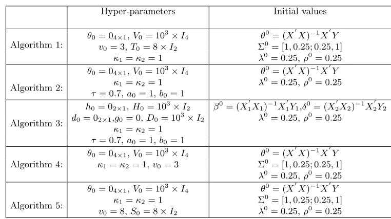
Table 1: Prior hyper-parameters and Initial Values

Hyper-parameters Initial values

Algorithm 1: θ

0= 04×1,V0= 103×I4 θ0 = (X

′

X)−1

X′Y v0= 3,T0= 8×I2 Σ

0

= [1,0.25; 0.25,1]

κ1=κ2= 1 λ0= 0.25,ρ0= 0.25

Algorithm 2:

θ0= 04×1,V0= 103×I4 θ0 = (X

′

X)−1

X′Y κ1=κ2= 1 λ

0

= 0.25,ρ0

= 0.25

τ= 0.7,a0= 1,b0= 1

Algorithm 3:

h0 = 02×1,H0= 103×I2 β0= (X

′

1X1)−1X

′

1Y1,δ0= (X

′

2X2)−1X

′

2Y2

d0= 02×1,g0= 0,D0= 103×I2 λ0= 0.25,ρ0= 0.25

κ1=κ2= 1

τ= 0.7,a0= 1,b0= 1

Algorithm 4:

θ0= 04×1,V0= 103×I4 θ0 = (X

′

X)−1_X′

Y κ1=κ2 = 1,v0= 3 Σ0= [1,0.25; 0.25,1]

λ0

= 0.25,ρ0

= 0.25

Algorithm 5:

θ0= 04×1,V0= 103×I4 θ0 = (X

′

X)−1_X′

Y κ1=κ2= 1 Σ0= [1,0.25; 0.25,1]

v0= 8,S0= 8×I2 λ 0

= 0.25,ρ0

= 0.25

15

4

Simulation Study

To evaluate the finite sample properties of Gibbs samplers in Algorithms 1-5, we design a simulation study in this section. We consider the following data generating process (DGP):

Y⋆

1

Y₂⋆

=

X1 0n×k2

0n×k1 X2

β δ

+

S−1_(λ)ε 1

R−1(ρ)ε2

. (4.1)

where X1 = (l

′

n, X

′

1,1)

′

with β = (β1, β2)

′

, and X2 = (l

′

n, X

′

2,1)

′

with δ = (δ1, δ2)

′

. The exogenous variableX1,1 consists of random draws fromU(0,1) whereasX2,1 is generated fromN(0,1).16 The

innovations are generated from the bivariate normal distribution according to

ε1i

ε2i

∼N 0

0

,

1 0.3

0.3 1.2 (4.2)

for i = 1, . . . , n. Hence, ̺ = 0.25. For the true parameter values, we set (δ1, δ2)

′

= (0.4,1.2)′, and β2 = 2. We use β1 to control the amount of the sample selection in the model. We set β1 =

−0.2 to generate 25% censuring. We consider (λ, ρ) ={(0.1,0.1),(0.4,0.4)} for the autoregressive parameters to allow for weak and moderate dependence in the error processes.

The row normalized W and M are based on the interaction scenario described in Liu and Lee, (2010). Both matrices are block diagonal matrices where each block represents the interaction structure of a group. Let the total sample involve R groups where the rth group has the groups size mr. We consider an experiment where R is set to 30. We allow mr to vary across R groups

by randomly assigning a value from the set of integers {10,11,12,13,14,15} to each group size. Therefore, the total number of observations nvaries between 300 and 450. The weight matrix Wr

for therth group is generated in two steps. First, an integer valueτir is uniformly drawn from the

set of integer values{1,2,3,4}. Then, ifτir+i≤mr, the (i+ 1)th, . . . ,(i+τir)th elements of the

ith row of Wr are set to one and the rest of the elements in the ith row are set to zero. On the

other hand, if τir +i > mr, the first (τir+i−mr) entries of the ith row are set to one and the

other elements of theith row are set to zero. Then,W =M = Diag(W1, . . . , WR).

The hyper-parameter values and the initial parameter values we used in the simulation are stated in Table 1. These values are close to those used in Imai and van Dyk, (2005) in a simulation for a multinomial probit model. In Algorithms 2 and 3, we setτ = 0.7, which generates a relatively diffuse prior for the correlation coefficient between ε1i and ε2i.17 Finally, we run each MCMC

algorithm for 60000 iterations. The first 10000 draws are discarded as a burn in period.

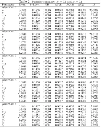
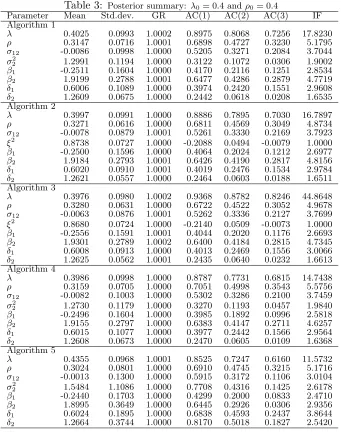
4.1 Simulation Results

The simulation results are presented in Tables 2-3, and Figures 1 – 4. We compare point estimates to gauge statistical inference implied by each algorithm in Tables 2 and 3. We provide (i) the mean of sampled draws, i.e., the estimated posterior means, (ii) the standard deviations of sampled draws (Std.dev.) and (iii) some other convergence diagnostics. The convergence diagnostics include, the Gelman-Rubin (GR) statistic, the first three lag-correlations in sampled draws (denoted by AC(1),

16

Pace et al., (2012) show that the explanatory variables used in applied studies exhibit spatial dependence. As shown in Pace et al., (2012), the spatial dependence among regressors can also effect the performance of the likelihood-based estimators. It will be interesting to see the effect of spatial dependence among regressors on the Bayesian estimator. This issue is raised by a referee and can be explored in future studies.

17

Table 2: Posterior summary: λ0= 0.1 andρ0= 0.1

Parameter Mean Std.dev. GR AC(1) AC(2) AC(3) IF Algorithm 1

λ 0.0836 0.1586 1.0006 0.9320 0.8684 0.8095 26.4242

ρ 0.1407 0.0761 1.0000 0.6840 0.4657 0.3181 5.2606

σ12 -0.0006 0.0923 1.0000 0.4730 0.2808 0.1680 3.2418

σ2

2 1.2653 0.1084 1.0000 0.2538 0.0710 0.0149 1.6795

β1 -0.1066 0.1429 1.0000 0.4552 0.2283 0.1279 2.9592

β2 1.8529 0.2798 1.0002 0.6312 0.4180 0.2864 4.7646

δ1 0.5266 0.0841 1.0000 0.3530 0.2005 0.1231 2.5820

δ2 1.2549 0.0685 1.0000 0.2609 0.0652 0.0239 1.6998

Algorithm 2

λ 0.0840 0.1603 1.0003 0.9364 0.8770 0.8218 27.0106

ρ 0.1459 0.0659 1.0000 0.6888 0.4707 0.3192 5.0085

σ12 0.0030 0.0822 1.0000 0.4763 0.2836 0.1720 3.2778

ξ2

0.8752 0.0696 1.0000 -0.1739 0.0305 -0.0045 1.0000

β1 -0.1070 0.1426 1.0000 0.4463 0.2192 0.1243 2.8113

β2 1.8563 0.2800 1.0000 0.6251 0.4071 0.2769 4.8148

δ1 0.5257 0.0704 1.0000 0.3557 0.2075 0.1192 2.5831

δ2 1.2556 0.0571 1.0000 0.2646 0.0719 0.0257 1.7243

Algorithm 3

λ 0.0856 0.1565 1.0002 0.9547 0.9125 0.8724 70.3474

ρ 0.1460 0.0647 1.0001 0.7127 0.5080 0.3624 5.8613

σ12 0.0038 0.0816 1.0000 0.4660 0.2713 0.1636 3.2068

ξ2

0.8689 0.0691 1.0000 -0.1770 0.0413 -0.0055 1.0000

β1 -0.1071 0.1438 1.0001 0.4447 0.2186 0.1179 2.8074

β2 1.8569 0.2806 1.0001 0.6222 0.4069 0.2728 4.6321

δ1 0.5248 0.0703 1.0000 0.3576 0.2019 0.1153 2.5566

δ2 1.2560 0.0571 1.0001 0.2628 0.0688 0.0221 1.7075

Algorithm 4

λ 0.0819 0.1566 1.0008 0.9617 0.9251 0.8900 51.7106

ρ 0.1409 0.0760 1.0001 0.6945 0.4835 0.3391 5.4550

σ12 0.0012 0.0931 1.0000 0.4767 0.2775 0.1648 3.1767

σ2

2 1.2414 0.1061 1.0000 0.2480 0.0651 0.0190 1.6643

β1 -0.1067 0.1422 1.0000 0.4426 0.2140 0.1125 2.7783

β2 1.8545 0.2802 1.0000 0.6259 0.4100 0.2770 4.7014

δ1 0.5262 0.0833 1.0000 0.3520 0.2032 0.1211 2.5676

δ2 1.2548 0.0681 1.0000 0.2657 0.0750 0.0209 1.7232

Algorithm 5

λ 0.2804 0.1427 1.0002 0.9029 0.8132 0.7333 17.8891

ρ 0.1427 0.0825 1.0003 0.7197 0.5149 0.3655 5.7368

σ12 0.0091 0.1176 1.0000 0.5323 0.2566 0.0676 2.6462

σ2

2 1.5528 1.1383 1.0000 0.7511 0.3920 0.1017 2.5470

β1 -0.0835 0.1554 1.0000 0.4409 0.2074 0.0900 2.5324

β2 1.7992 0.3668 1.0000 0.6350 0.2729 0.0058 2.8274

δ1 0.5354 0.1672 1.0000 0.6900 0.4335 0.1940 3.6725

δ2 1.2826 0.3755 1.0001 0.8096 0.4779 0.1509 2.6257

AC(2), and AC(3)), and the inefficiency factors (IF). The inefficiency factor (or autocorrelation time) is defined as the ratio of the squared numerical standard errors to the variance of the posterior mean based on the hypothetical independent draws (Chib, 2001, p. 3580).18 _{An efficient sampler}

would generate a sequence of sampled draws with a small IF close to 1.

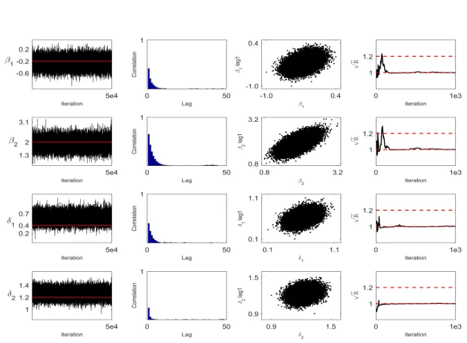
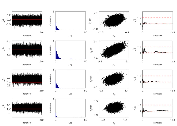
We also provide several graphical summaries of draws in Figures 1 – 4 to compare algorithms in terms of convergence and mixing properties of the corresponding Markov chains. For the sake of brevity, we only provide the figures for Algorithms 1 and 4 for the case of{λ, ρ}={0.4,0.4}.19 These figures include the convergence plots (or time series plots), the autocorrelation plots, the lag-one scatter plots, and the Gelman and Rubin, (1992)’s √R statistic. The convergence plots in these figures for a parameter simply show all draws generated by the samplers against iterations. The autocorrelation plots provide a simple visual inspection of the lag-correlation in sampled draws

18

It is calculated as IF(θ) = 1 + 2PM−1

k=1 1−

k M

ρk, where M is the total number of draws, andρk is the lag k

sample autocorrelation.

19

Table 3: Posterior summary: λ0= 0.4 andρ0= 0.4

Parameter Mean Std.dev. GR AC(1) AC(2) AC(3) IF Algorithm 1

λ 0.4025 0.0993 1.0002 0.8975 0.8068 0.7256 17.8230

ρ 0.3147 0.0716 1.0001 0.6898 0.4727 0.3230 5.1795

σ12 -0.0086 0.0998 1.0000 0.5205 0.3271 0.2084 3.7044

σ2

2 1.2991 0.1194 1.0000 0.3122 0.1072 0.0306 1.9002

β1 -0.2511 0.1604 1.0000 0.4170 0.2116 0.1251 2.8534

β2 1.9199 0.2788 1.0001 0.6477 0.4286 0.2879 4.7719

δ1 0.6006 0.1089 1.0000 0.3974 0.2420 0.1551 2.9608

δ2 1.2609 0.0675 1.0000 0.2442 0.0618 0.0208 1.6535

Algorithm 2

λ 0.3997 0.0991 1.0000 0.8886 0.7895 0.7030 16.7897

ρ 0.3271 0.0616 1.0000 0.6811 0.4569 0.3049 4.8734

σ12 -0.0078 0.0879 1.0001 0.5261 0.3330 0.2169 3.7923

ξ2

0.8738 0.0727 1.0000 -0.2088 0.0494 -0.0079 1.0000

β1 -0.2500 0.1596 1.0000 0.4064 0.2024 0.1212 2.6977

β2 1.9184 0.2793 1.0001 0.6426 0.4190 0.2817 4.8156

δ1 0.6020 0.0910 1.0001 0.4019 0.2476 0.1534 2.9784

δ2 1.2621 0.0557 1.0000 0.2464 0.0603 0.0188 1.6511

Algorithm 3

λ 0.3976 0.0980 1.0002 0.9368 0.8782 0.8246 44.8648

ρ 0.3280 0.0631 1.0000 0.6722 0.4522 0.3052 4.9678

σ12 -0.0063 0.0876 1.0001 0.5262 0.3336 0.2127 3.7699

ξ2

0.8680 0.0724 1.0000 -0.2140 0.0509 -0.0073 1.0000

β1 -0.2556 0.1591 1.0001 0.4044 0.2020 0.1176 2.6693

β2 1.9301 0.2789 1.0002 0.6400 0.4184 0.2815 4.7345

δ1 0.6008 0.0913 1.0000 0.4013 0.2469 0.1556 3.0066

δ2 1.2625 0.0562 1.0001 0.2435 0.0640 0.0232 1.6613

Algorithm 4

λ 0.3986 0.0998 1.0000 0.8787 0.7731 0.6815 14.7438

ρ 0.3159 0.0705 1.0000 0.7051 0.4998 0.3543 5.5756

σ12 -0.0082 0.1003 1.0000 0.5302 0.3286 0.2100 3.7459

σ2

2 1.2730 0.1179 1.0000 0.3270 0.1193 0.0457 1.9840

β1 -0.2496 0.1604 1.0000 0.3985 0.1892 0.0996 2.5818

β2 1.9155 0.2797 1.0000 0.6383 0.4147 0.2711 4.6257

δ1 0.6015 0.1077 1.0000 0.3977 0.2442 0.1566 2.9564

δ2 1.2608 0.0673 1.0000 0.2470 0.0605 0.0109 1.6368

Algorithm 5

λ 0.4355 0.0968 1.0001 0.8525 0.7247 0.6160 11.5732

ρ 0.3024 0.0801 1.0000 0.6910 0.4745 0.3215 5.1716

σ12 -0.0013 0.1300 1.0000 0.5915 0.3172 0.1106 3.0104

σ2

2 1.5484 1.1086 1.0000 0.7708 0.4316 0.1425 2.6178

β1 -0.2440 0.1703 1.0000 0.4299 0.2000 0.0833 2.4710

β2 1.8995 0.3649 1.0000 0.6445 0.2926 0.0306 2.9356

δ1 0.6024 0.1895 1.0000 0.6838 0.4593 0.2437 3.8644

δ2 1.2664 0.3744 1.0000 0.8170 0.5018 0.1827 2.5420

and can be used to assess the mixing properties of the sampler. Low autocorrelation in sampled draws means that the sampler is expected to converge to the posterior distribution more quickly. Hence, slowly decaying autocorrelations in these figures indicate inefficiencies for a sampler. The

√

R statistic is defined as the ratio of the between-chain variance and the within-chain variance; and values close to one indicate acceptable mixing.

We provide the salient features of our results in the following list.

1. The results in Tables 2 and 3 indicate that the estimated posterior means of autoregressive parameters are close to true parameter values, except in the case of Algorithm 5 forλ. These results become visually available through the convergence plots provided in Figures 1 – 4. The sampled draws generated for ρ are slightly off-centered from the true parameter value.

2. The Bayesian point estimates forσ12are far away from the true value in all algorithms. As can

Figure 1: Algorithm 1

Figure 3: Algorithm 4

the estimates for ξ2 _{deviate substantially from the true value. Algorithms 1 and 4 report}

estimates ofσ2

2 that are close to the true value, while Algorithm 5 does not.

3. Although all algorithms report estimates forβ1 andδ2 that are close to the true values, there

is some deviations in the case ofβ2andδ1. Overall, the deviation between estimated posterior

means and the true values is relatively smaller in Table 2, and the Bayesian estimator based on Algorithms 1 and 4 performs relatively better in both tables.

4. To give an overall picture on the deviation between the estimated posterior means and the true parameter values, we calculate average deviations over all parameters from Tables 2 and 3. In Table 2, the average absolute deviation is (i) 0.1056 from Algorithm 1, (ii) 0.1264 from Algorithm 2, (iii) 0.1268 from Algorithm 3, (iv) 0.1023 from Algorithm 4, and (v) 0.1752 from Algorithm 5. In Table 3, we have the average absolute bias of (i) 0.1110 from Algorithm 1, (ii) 0.1266 from Algorithm 2, (iii) 0.1264 from Algorithm 3, (iv) 0.1078 from Algorithm 4, and (v) 0.1495 from Algorithm 5. Hence, Algorithms 1 and 4 performs relatively better in both tables.

5. The standard deviations reported in both tables are close to each other for the first four algorithms. The standard deviations reported for Algorithm 5 are slightly larger, especially in the case ofσ2₂.

6. The reported Gelman-Rubin (GR) statistic, the IF statistics, the autocorrelation plots, the lag-one scatter plots and the √R statistics can be used to assess the mixing properties of samplers. The Gelman-Rubin statistics in Tables 2 and 3 suggest that the Markov chains are mixing well. The √R statistics in Figures 1 – 4 stabilize near one quickly. The inefficiency factor (IF) statistics are very similar across algorithms except for the case ofλ. In particular, the autocorrelation plots and lag-one scatter plots for λ in Figures 1 – 4 indicate that the autocorrelation among draws decays slowly, leading to large values of IF in all algorithms. Overall our results indicate that there is no substantial differences among algorithms in terms of mixing properties.20

5

Empirical Illustration

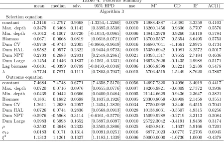
For the empirical illustration, we use the application in the area of natural resource economics considered in Flores-Lagunes and Schnier, (2012). In this application, the authors model the spatial production within a fishery with a spatial sample selection model. The data set is collected from the Pacific cod fishery, located in the Eastern Bering Sea of Alaska. Among the groundfish fisheries of Alaska, the Pacific cod fishery is the second largest one with landings valued at more than 185 million dollars in 2012. For production purposes, the fishery is divided into 90 spatially different locations. The catch per unit effort (CPUE) which is measured as the metric tons of fish caught during the year 1997 in a fishing fleet is used to analyze the productivity and efficiency

20