Dealing with Misspecification in DSGE Models: A Survey

Munich Personal RePEc Archive

Dealing with Misspecification in DSGE

Models: A Survey

Paccagnini, Alessia

University College Dublin, Michael Smurfit Graduate Business

School

24 November 2017

Online at

https://mpra.ub.uni-muenchen.de/82914/

Dealing with Misspeci…cation in DSGE Models: A Survey

Alessia Paccagnini

November 24, 2017

Abstract

Dynamic Stochastic General Equilibrium (DSGE) models are the main tool used in Academia and in Central Banks to evaluate the business cycle for policy and forecasting analyses. Despite the recent

advances in improving the …t of DSGE models to the data, the misspeci…cation issue still remains. The aim of this survey is to shed light on the di¤erent forms of misspeci…cation in DSGE modeling and how the researcher can identify the sources. In addition, some remedies to face with misspeci…cation are

discussed.

JEL CODES: C11, C15, C32

KEYWORDS: DSGE Models, Misspeci…cation, Estimation, Bayesian Estimation

"Essentially, all models are wrong, but some are useful"

George Box and Norman Draper in "Empirical Model-Building and Response Surfaces" (1987, pag.424)

"A well-de…ned statistical model is one whose underlying assumptions are valid for the data chosen"

Aris Spanos in "The Simultaneous-Equations Model Revisited: Statistical Adequacy and Identi…cation"

(1990, pag.89)

1

Introduction

Dynamic Stochastic General Equilibrium (DSGE) models are the workhorse of modern macroeconomists

in both Academia and policymaker institutions, such as Central Banks (Kydland and Prescott, 1982 and

Rotemberg and Woodford, 1997). Introduced to satisfy the Lucas critique (Lucas, 1976), with respect to

structural macroeconometrics models, DSGE describe the business cycle using micro-economic foundations.

Thanks to these features, these models are particularly suited for policy evaluations and for forecasting

analysis of the key economic indicators (output, in‡ation, and short-term interest rate), as illustrated in

the works of Smets and Wouters (2003, 2004, and 2007), Del Negro and Schorfheide (2004), Christiano,

Eichenbaum, and Evans (2005), and Adolfson, Laséen, Lindé, and Villani (2008) among others.

Despite these recent advances in improving the …t of DSGE models to the data, the misspeci…cation issue

still remains. A growing number of papers have discussed the important role of misspeci…cation in DSGE

models and how we can identify the sources of misspeci…cation. In particular, the recent Great Recession

has brought new importance to investigate about the structural economic model’s di¢culties in explaining

the data to make policy evaluation and for forecasting purposes.

This survey aims to shed light on this issue and reply to the following questions:

What does the misspeci…cation mean in a DSGE model? How can we identify the sources of

misspeci…-cation? What are the main approaches to face with misspeci…misspeci…-cation?

The review starts examining the standard New Keynesian DSGE model à la Smets and Wouters (2007)

which is the benchmark model to explain the business cycle behavior in the current DSGE modeling literature.

After that, we discuss the di¤erent forms of misspeci…cation the researcher can face in using the benchmark

model to make policy evaluation and forecasting analysis. So far, the literature does not propose a unique

de…nition of misspeci…cation. We can distinguish four forms of misspeci…cation: a) Misspeci…cation in the

State-Space Representation, b) Misspeci…cation in Parameters, c) Misspeci…cation in the Assumptions of the

DSGE model, and d) Misspeci…cation in Computational Methods. Furthermore, each form of misspeci…cation

includes di¤erent aspects. Misspeci…cation in the State-Space Representation relies on three problems:

Misspeci…cation and Model Features, Misspeci…cation and Shocks, and Misspeci…cation of the Statistical

Representation. Instead, Misspeci…cation in Parameters refers to the role of the parameter stability and

the identi…cation in DSGE misspeci…cation. Meanwhile, Misspeci…cation in the Assumptions refers to the

hypothesis of rational expectations and of linearity. Last but not least, Misspeci…cation in Computational

Methods refers to estimation of the posterior in the DSGE modeling.

The review also delineates the approaches to detect the sources of misspeci…cation, focusing on Monti

(2015), Inonue, Kuo, and Rossi (2017), Canova and Matthes (2017), and Den Haan and Dreschel (2017).

After that, we discuss about the econometric methods used to deal with the DSGE misspeci…cations. In

particular, we focus on the (additive and hierarchical) hybrid DSGE models as shown in Schorfheide (2013).

The remainder of the paper is organized as follows. Section 2 illustrates the medium scale DSGE model à

la Smets and Wouters (2007). Section 3 discusses the di¤erent forms of misspeci…cation. Section 4 overviews

the methodologies to detect the sources of misspeci…cation. Section 5 shows how the researcher can deal

with DSGE misspeci…cation using hybrid models. Section 6 summarizes the …ndings and provides concluding

2

Medium Scale Model: Smets and Wouters (2007)

The Smets and Wouters (2007) model is a medium scale model which features sticky nominal price and wage

contracts, habit formation, variable capital utilization and investment adjustment costs. The closed economy

consists of households, labor unions, labor packers, a productive sector, and a monetary policy authority.

Households consume, accumulate government bonds and supply labor. A labor union di¤erentiates labor

and sets wages in a monopolistically competitive setup. Competitive labor packers buy labor services from

the union, package and sell them to intermediate goods …rms. Output is produced in several steps, including

a monopolistically competitive sector with producers facing price rigidities. The monetary policy authority

sets the short-term interest rate according to a Taylor rule. As described in Smets and Wouters (2007) and

Bekiros and Paccagnini (2014), the model is represented by the following equations.

The demand side of the economy is composed by consumption (ct), investment (it), capital utilization

(zt), and government spending"gt = g" g

t 1+ g gt+ ga at which is assumed to be exogenous.

The total output (yt) is represented by:

yt=cyct+iyit+zyzt+"gt; (1)

wherecyis the steady-state share of consumption in output and equals (1 gy iy), wheregy andiy are

respectively the steady-state exogenous spending-output ratio and investment-output. Instead,zy =Rkky,

whereRk _{is the steady-state rental rate of capital, andk}

y is the steady-state capital-output ratio.

The consumption Euler equation evolves as:

ct =

=

1 + = ct 1+ 1 =

1 + = Etct+1+ (2)

( c 1) WhL =C c(1 + = )

(lt Etlt+1)

(1 = )

c(1 + = )

(rt Et t+1+"bt);

whereltis the hours worked,rtis the nominal interest rate, and tis the rate of in‡ation. If the degree of

habits is zero ( = 0) and c= 1, Equation (2) reduces to the standard forward looking consumption Euler

equation. The disturbance is assumed to follow a …rst-order autoregressive process with an IID-Normal error

term: "b

t= b"bt 1+ bt:

it =

1

1 + (1 c)it 1+ 1

1

1 + (1 c) Etit+1+ (3)

1

(1 + (1 c)) 2'qt+"

i t;

where it denotes the investment and qt is the real value of existing capital stock (Tobin’s Q). ' is

the steady-state elasticity of the capital adjustment cost function, and is the discount factor applied by

households. The investment-speci…c technology process follows a …rst-order autoregressive process with an

IID-Normal error term: "i

t= i"it 1+ it:

The arbitrage equation for the value of capital is given by:

qt = (1 )Etqt+1+ (1 (1 ))Etrtk+1 (4)

(rt Et t+1+"bt);

where rk

t = (kt lt) +wt denotes the real rental rate of capital which is negatively related to the

capital-labour ratio and positively to the real wage.

On the supply side of the economy, the aggregate production function is de…ned as:

yt= p( kst+ (1 )lt+"at); (5)

where p and are respectively one plus the share of …xed costs in production and the share of capital

in production. The total factor productivity follows a …rst-order autoregressive process: "a

t = a"at 1+ at:

ks

t represents capital services which is a linear function of lagged installed capital (kt 1) and the degree

of capital utilization, ks

t =kt 1+zt: Capital utilization is proportional to the real rental rate of capital,

zt= 1 rkt, where is a positive function of the elasticity of the capital utilization adjustment cost function

and normalized from zero (in equilibrium the rental rate on capital is constant) to one (the utilization of

capital is constant).

The accumulation process of installed capital is simply described as:

kt=

1

kt 1+

1 +

it+ 1

(1 )

1 + (1 c) 2_{' "}i

t; (6)

Monopolistic competition within the production sector and Calvo-pricing constraints gives the

t = p

1 + (1 c)

p t 1+

(1 c)

1 + (1 c)

p

Et t+1 (7)

1 1 + (1 c)

p

1 (1 c)

p(1 p) p( p 1)"p+ 1

p t+"

p t;

where pt = (kts lt) wtis the marginal cost of production and the price mark-up disturbance follows

an ARMA(1,1)1 _process"p t = p"

p t 1+

p t p

p

t 1;where

p

t is an IID-Normal price mark-up shock. If the

degree of indexation to past in‡ation is zero, p= 0, the Equation (7) becomes a standard forward-looking

Phillips curve. The speed of adjustment depends on the degree of price stickness ( p), the curvature of

the Kimball goods market aggregator ("p), and the steady-state mark-up which is related in equilibrium to

( p 1), the share of …xed costs in production.

Monopolistic competition in the labour market also produces a similar wage New-Keynesian Phillips

curve:

wt = 1

1 + (1 c)wt 1+

(1 c)

1 + (1 c)(Etwt+1 Et t+1) (8)

1 + (1 c)

w

1 + (1 c) t+

w

1 + (1 c) t 1

1 1 + (1 c)

1 (1 c)

w(1 w)

( w( w 1)"w+ 1) w t +"wt;

where w

t =wt llt+₁ 1₌ (ct = ct 1)is the households’ marginal bene…t of supplying an extra unit

of labour service and the wage mark-up shock is an ARMA(1,1)2 _process,"w

t = w"wt 1+ wt w wt 1;where

w

t is an IID-Normal error term. If the degree of indexation to past in‡ation is zero, w= 0, the Equation (8)

does not depend on lagged in‡ation. The speed of adjustment depends on the degree of wage stickness ( w),

the curvature of the Kimball labour market aggregator ("w), and the steady-state labour market mark-up

( w 1).

The model is closed by the Taylor rule:

rt= rt 1+ (1 ) [r t+rY(yt ytp)] +r y (yt ytp) (yt 1 ypt 1) +"rt; (9)

where ytp is the ‡exible price level of output and "rt = r"rt 1+ rt follows a …rst-order autoregressive

process with an IID-Normal error term.

Equations (1) to (9) determine 14 endogenous variables: yt; ct; it; qt; kts; kt; zt; rkt; p

t; wt; t; wt;

lt and rt: The stochastic behaviour of the system of linear rational expectations equations is driven by 7

exogenous disturbances: total factor productivity ("at), investment-speci…c technology ("it), risk-premium

("b

t), exogenous spending ("gt), price mark-up ("pt), wage mark-up ("wt), and monetary policy shock ("rt).

The model can be solved by applying the algorithm proposed by Sims (2002). As discussed in Chib

and Ramamurthy (2010), the vector of states has a 53 dimensional, given the sticky price-wage and ‡exible

price-wage settings (in asterisks):

~

Zt= (yt; kst; lt; rkt; wt; t; pt; ct; rt; zt; qt; it; kt; wt; Et t+1; Etct+1; Etlt+1; Etqt+1; Etrkt+1; Etit+1;

Etwt+1; yt 1; ct 1; it 1; wt 1; uat; ubt; u g

t; uit; urt; u p t; uwt; "

p

t; "wt; yt; kts ; lt; rkt ; wt; t; p

t ; ct; rt; zt; qt;

it; kt; wt ; Etct+1; Etlt+1; Etqt+1; Etrtk+1; Etit+1; yt 1):

The vector of innovations:

t= "at; "it; "bt; " g t; "

p

t; "wt; "rt

and the vector of the endogenous rational expectations errors:

t= ( t Et 1 t; ct Et 1ct; lt Et 1lt; qt Et 1qt; rkt Et 1rtk; it Et 1it; wt Et 1wt; ct Et 1ct;

lt Et 1lt; qt Et 1qt; rtk Et 1rkt ; it Et 1it):

Therefore the previous set of Equations, (1) - (9), can be recasted into a set of matrices( 0; 1; C; ; )

accordingly to the de…nition of the vectorsZ~t and t:

0Z~t=C+ 1Z~t 1+ t+ t: (10)

The following transition equation is the solution written as policy function:

~

Zt=T( ) ~Zt 1+R( ) t; (11)

and in order to provide the mapping between the observable data and those computed as deviations from

Yt= 2 6 6 6 6 6 6 6 6 6 6 6 6 6 6 6 6 6 4

lnyt

lnct

lnit

lnwt

lnlt

lnPt

lnRat

3 7 7 7 7 7 7 7 7 7 7 7 7 7 7 7 7 7 5 = 2 6 6 6 6 6 6 6 6 6 6 6 6 6 6 6 6 6 4 l r 3 7 7 7 7 7 7 7 7 7 7 7 7 7 7 7 7 7 5 + 2 6 6 6 6 6 6 6 6 6 6 6 6 6 6 6 6 6 4

yt yt 1 ct ct 1 it it 1 wt wt 1

lt t rt 3 7 7 7 7 7 7 7 7 7 7 7 7 7 7 7 7 7 5 ;

where ln denotes 100 times log and ln refers to the log di¤erence. = 100( 1) is the common

quarterly trend growth rate to real GDP, consumption, investment, and wages. Instead, = 100( 1)

is quarterly steady-state in‡ation rate,r= 4 100( 1 c _{1) is the steady-state nominal interest rate,}

andl is the steady-state hours worked, which is normalized to be equal to zero. We can write the following equation:

Yt= 0( ) + 1( ) ~Zt+vt; (12)

whereYt= ( lnyt; lnct; lnit; lnwt;lnlt; lnPt;lnRat)

0

,vt= 0and 0and 1are de…ned accordingly.

The matricesT, R, 0and 1are in function of the structural parameters in the model.

The linearized state-space representation of the Smets and Wouters (2007) (but in general of any DSGE

model with no-time-varying parameters ( )) is as follows:

Yt = 0( ) + 1( ) ~Zt+vt; (13)

~

Zt = T( ) ~Zt 1+R( ) t ,

where Yt is a vector of (k 1) observables, such as aggregate output, in‡ation, and interest rates.

This vector represents the measurement equation. Instead, the vector Z~t (n 1) contains the unobserved

exogenous shock processes and the potentially unobserved endogenous state variables of the model. The

model speci…cation is completed by setting the initial state vectorZ0~ and making distributional assumptions for the vector of innovations t(E[ t] = 0; E

h

t

0

t

i

=I andE[ t t j] = 0forj6= 0). vtis the measurement

error.

Over the last few years, Bayesian estimation of DSGE models has become very popular. As discussed

estimation is system-based and …ts the solved DSGE model to a vector of aggregate time series, as opposed

to the Generalized Method of Moments (GMM) which is based on equilibrium relationships, such as the

Euler equation for the consumption or the monetary policy rule. Second, Bayesian estimation is based on

the likelihood function generated by the DSGE model rather than the discrepancy between DSGE responses

and VAR impulse responses. Third, prior distributions can be used to incorporate additional information

into the parameter estimation.

On a theoretical level, the Bayesian estimation takes the observed data as given, and treats the parameters

of the model as random variables. In general terms, the estimation procedure involves solving the linear

rational expectations model described above and the solution is written in Equation (13). After that, the

Kalman Filter is applied to develop the likelihood function. Prior distributions are important to estimate

DSGE models. According to An and Schorfheide (2007), priors might downweigh regions of the parameter

space that are at odds with observations which are not contained in the estimation sample. Priors could

add curvature to a likelihood function that is (nearly) ‡at for some parameters, given a strong in‡uence

to the shape of the posterior distribution. Posterior distribution of the structural parameters is formed

by combining the likelihood function of the data with a prior density, which contains information about

the model parameters obtained from the other sources (microeconometrics, calibration, and cross-country

evidence), thus allowing to extend the relevant data beyond the time series which are used as observables.

Numerical methods such as Monte-Carlo Markov-Chain (MCMC) are used to characterize the posterior with

respect to the model parameters.3

3

Forms of Misspeci…cation

The statistical representation in Equation (13) could be misspeci…ed. As stated in Fernández-Villaverde,

Rubio-Ramirez, and Schorfheide (2016), model misspeci…cation can be interpreted as a violation of the

cross-coe¢cient restrictions embodied in the mapping from the DSGE model parameters into the system

of matrices of the state-space representation. Canova and Matthes (2017) and Canova (2017) discusses

about the misspeci…cation referring not only about the state-space representation but adding issues about

parameters in the misspeci…ed model. So far, in the DSGE modeling literature there is not a unique de…nition

of misspeci…cation. This survey sheds light distinguishing four forms of misspeci…cation: a) Misspeci…cation

in the State-Space Representation, b) Misspeci…cation in Parameters, c) Misspeci…cation in the Assumptions

of the DSGE model, and d) Misspeci…cation in Computational Methods.

3_{See Smets and Wouters (2003, 2007), An and Schorfheide (2007), and Herbst and Schorfheide (2015) for more details on}

The …rst form of misspeci…cation(a) ) refers to the de…nition described in Fernández-Villaverde,

Rubio-Ramirez, and Schorfheide (2016), adding the second form of misspeci…cation (b) ), we can refer to the general

de…nition of misspeci…cation discussed in Canova and Matthes (2017) and Canova (2017).

Moreover, each form of misspeci…cation includes di¤erent aspects. Misspeci…cation in the State-Space

Representation relies on three problems: Misspeci…cation and Model Features, Misspeci…cation and Shocks,

and Misspeci…cation of the statistical representation. Instead, Misspeci…cation in Parameters refers to the

role of the parameter stability and the identi…cation in DSGE misspeci…cation. Meanwhile, Misspeci…cation

in the Assumptions refers to the hypothesis of rational expectations and of linearity. Last but not least,

Misspeci…cation in Computational Methods refers to estimation of the posterior in the DSGE modeling.

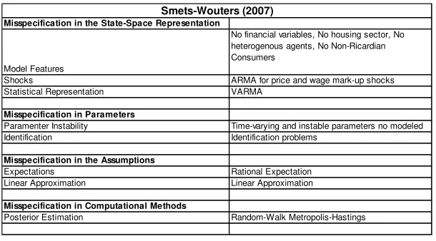
Table 1 summarizes the misspeci…cation aspects referring to the Smets and Wouters (2007) model.

3.1

Misspeci…cation in the State-Space Representation

1) Misspeci…cation and Model Features. DSGE models, as any other models, are a stylized picture

of reality. Small scale DSGE and medium scale DSGE are often used for policy analysis and forecasting

comparisons. Some models could be misspeci…ed since they do not include relevant variables.

For example, Smets and Wouters (2007) ignore …nancial and housing markets which are relevant variables

to explain the shocks dynamics, in particular during crisis periods. Furthermore, …scal sector and labor

market are stylized and not properly modelled in the Smets and Wouters (2007). Recently, these medium

scale models have been criticized for their limitation to explain the Great Recession4_{. Del Negro and}

Schorfheide (2013) is an example of improvement of the …t of structural economic framework during the

crisis, including in‡ation expectations, …nancial frictions, and interest rate spreads.

In addition, there are several model features made by researchers to simplify the theoretical model, such

as constant real interest rate, quadratic preferences in consumption, homogeneous agents, and exogenous

labour income. But some of these elements could be relaxed to improve the matching between the theory and

the data. For example, several models show interesting results using heterogeneous agents (see Colander,

Howitt, Kirman, Leijonhufvud and Mehrling, 2008, Den Haan, 2010, Massaro, 2013, McKay and Reis, 2016,

and Kaplan, Moll, and Violante, 2017 among others). In terms of consumers, DSGE models could incorporate

a fraction of Non-Ricardian households who do not hold any wealth and entirely consume their disposable

labor income in each period (the Limited Asset Market Participation hypothesis) (as discussed in theoretical

framework in Galí et al., 2004 and Bilbiie, 2008; and recently in empirical analysis in Albonico, Paccagnini,

and Tirelli, 2016 and 2017).

4_{Christiano, Eichenbaum, and Trabandt (2017) review the state of DSGE models before the …nancial crisis and how the role}

2) Misspeci…cation and Shocks. Usually, in a DSGE model the number of observable variables

matches the number of shocks to face with the non-singularity condition. The Smets and Wouters (2007)

model features seven observable variables which match seven exogenous disturbances: total factor

productiv-ity ("a

t), investment-speci…c technology ("it), risk-premium ("bt), exogenous spending ("gt), price mark-up ("pt),

wage mark-up ("w

t), and monetary policy shock ("rt). All shocks are modelled as white noise with exception

price and wage mark-ups which are modelled as ARMA processes.

Adding shocks has been always a common practice to improve the connection of the theoretical DSGE

with the observed data and there are several interesting contributions. Firstly, Sargent (1989) and Ireland

(2004) introduce serial correlated errors in measurement equations of the state-space representation of the

model. Recently, Canova, Ferroni, and Matthes (2014) propose two methods to choose the variables to

be used in the estimation of the structural parameters of a DSGE model which su¤ers from singularity.

The …rst method allows to select the vector of observables which optimizes the parameter identi…cation;

the second one allows to select the vector which minimizes the gap between the singular and non-singular

model. Meanwhile, Ferroni, Grassi, and Léon-Ledesma (2017) focus on the di¤erence between "primal" and

"no primal", called "non-existent" shocks. Typically DSGE models are estimated assuming the existence

of certain "primal" or structural shocks which drive the business cycle. Ferroni, Grassi, and Léon-Ledesma

(2017) analyze the consequences of estimating shocks which are "non-existent" and they propose a rigorous

method to select the structural or primal shocks driving macroeconomic uncertainty. They provide evidence

how forcing the existence of "non-existent" shocks generates a downward bias in the estimated internal

persistence of the DSGE model. They evidence how the researcher can avoid or reduce these distorsions

by allowing the covariance matrix of the structural shocks to be rank de…cient. To avoid the downward

bias, they propose to use normal or exponential priors (which include zero) for standard deviations together

with measurement error to avoid stochastic singularity. At the same time, Meyer-Gohde and Neuho¤ (2015)

discuss the importance of stochastic shocks in the misspeci…cation of DSGE models relying on an ARMA

set-up for them. They propose a Bayesian approach to estimate the order as well as the parameters of generalized

ARMA representations of exogenous driving forces within the DSGE. To make this generalization, they adopt

the Reversible Jump Markov Chain Monte Carlo (RJMCMC) methodology introduced by Green (1995).

3) Misspeci…cation of the Statistical Representation. Several research studies5 _{have challenged}

the validity of a Vector Autoregressive (VAR) or a Structural VAR (SVAR) as main tool for estimating and

studying the transmission mechanisms of macroeconomic shocks. In particular, linearization of DSGE with

…rst-order approximation made linear time series models such as VARs suitable for evaluating DSGE model

5_{Ravenna (2007), Liu and Theodoridis (2012), Giacomini (2013), Franchi and Vidotto (2013), Pagan and Robinson (2016),}

restrictions.

First, DSGE and VARs models can be related in an indirect inference or minimum-distance set-up in

which we assume that the DSGE model provides a realistic probabilistic representation of the data. Hence,

the researcher chooses the DSGE model parameters such that VAR coe¢cients or impulse response functions

realized from the actual data match those obtained from the DSGE model-simulated data as closely as

possible. The magnitude of the minimized discrepancy provides a measure of …t. This approach, of using

the VAR as an auxiliary model, was …rstly discussed in Smith (1993) and Cogley and Nason (1994).

Second, following Schorfheide (2000) who discusses the idea that the DSGE model is considered

(po-tentially) misspeci…ed, Del Negro and Schorfheide (2004) and Del Negro, Schorfheide, Smets, and Wouters

(2007a) introduce the DSGE-VAR, providing a hybrid model to combine the information derived from the

prior of the theoretical model with the time series properties through the VAR representation which

approx-imates the DSGE model. Chari, Kehoe, and McGrattan (2008) examine a stylized business cycle model and

…nd that the impulse response function (IRF) computed from a …nite-order VAR yields a poor

characteriza-tion of the true responses. Alike, in a study about the real business cycle (RBC) models, Erceg, Guerrieri,

and Gust (2005) evidence that the error associated with using a …nite-order VAR model can be large and

attribute this to small-sample error. In contrast, Ravenna (2007) discusses how a …nite-order SVAR model

can lead to inaccurate estimates of the true IRFs but points out that this may not be a small-sample

prob-lem. Moreover, Ravenna (2007) shows that the error derives from two separate sources: a "truncation bias"

and an "identi…cation bias". Recently, Poskitt and Yao (2017) provide a detailed theoretical examination

of the loss incurred when approximating a VAR(1) process by a …nite lag VAR(p) model. They name them: "estimation error" (the di¤erence between the estimated VAR(p) and its theoretical counterpart) and "approximation error" (the di¤erence between the theoretical minimum mean squared error VAR(p) approximation and the true VAR(1) process).

We have to point out that many DSGE models have a solution which is not compatible with a …nite

VAR representation, but they should be represented by a VARMA model as discussed in Giacomini (2013),

Franchi and Vidotto (2013), Pagan and Robinson (2016), and Morris (2016 and 2017) among others.

The Smets and Wouters (2007) has the price and wage mark-up shocks which are ARMA processes,

hence, this model is represented by a VARMA and the solution does not involve a …nite order VAR.

The DSGE model validation cannot rely on the VAR since the true statistical representation of a DSGE

model is not always a …nite order VAR. Hence, using the traditional modeling approach, we have several

weakness such as statistical misspeci…cation, non-identi…cation of deep parameters (of the optimizing model),

weak forecasting evaluation, and potentially misleading Impulse Response Functions (IRFs) as shown in

"non-invertibility" of the moving average representation implied by the model. When such representation is

not invertible, a VAR representation in terms of all of the structural shocks does not exist 6_.

Fernández-Villaverde, Rubio-Ramirez, Sargent and Watson (2007) derive a condition for the validity of VAR methods,

related to the state-space representation of the macroeconomy. The condition, known as the "Poor Man’s

Condition", implies fundamentalness of the corresponding moving average representation and the possibility

of recovering all of the structural shocks from a VAR.

Poudyal and Spanos (2016) contribute the literature presenting a rigorous statistical analysis to evaluate

the validity of the implicit statistical model. The failure of these tests evidences how the Normal VAR

representation is statistically misspeci…ed. They propose a Student’s t VAR model to overcome the problem

of the weak model validation. The Student’s t VAR model is also useful to identify the deep structural

parameters, and hence to improve the forecasting performance and the policy analysis through IRFs.

However, if the true statistical representation for a DSGE model is the VARMA, the natural counterpart

should the VARMA model. As stated in Morris (2016), VARMA representations of DSGE models are

currently not widely utilized7_.

3.2

Misspeci…cation in Parameters

1) Misspeci…cation and Parameter Instabilities. The Smets and Wouters (2007) model features

pa-rameters without instabilities, but DSGE empirical literature has discussed alternative approaches to deal

with the possible problem of parameters instabilities8_{.With Markov-switching DSGE framework, the}

re-searcher models and estimates the regime change in some of the key parameters (Bianchi, 2013, Foerster,

Rubio-Ramirez, Waggoner, and Zha, 2016, Eo and Kim, 2016). Similar to Markov-switching, Waggoner

and Zha (2012) estimate a Markov-switching mixture of two models: a DSGE model and a Bayesian VAR.

They …nd that the Markov-switching mixture model dominates both models and improves the …t. This

interesting approach is introduced to deal with misspeci…cation issues. A practical way to introduce the

parameter instabilities in a DSGE model, in particular in a forecasting exercise is shown in Kolasa and

Rubaszek (2015). They observe that central banks are used to re-estimate DSGE models only occasionally

but this practice might a¤ect the forecasting performance. Hence, they investigate how frequently models

6_{Lippi and Reichlin (1993), Alessi, Barigozzi, and Capasso (2011), Sims (2012), Liu and Theodoridis (2012), Leeper, Walker}

and Yang (2013), Beaudry, Fève, Guay, and Portier (2015), Forni and Gambetti (2016), Soccorsi (2016), Chen, Choi and Escanciano (2017), Forni, Gambetti, Lippi and Sala (2017a) and (2017b), and Forni, Gambetti, and Sala (2017) among others.

7_{An exception to this, Kascha and Mertens (2009) propose an interesting application about business cycle estimating a}

VARMA model.

8_{Villaverde, Guerrón-Quintana, and Rubio-Ramirez (2010), Inoue and Rossi, (2011), Caldara,}

should be re-estimated so that the accuracy of forecasts they generate may be una¤ected. Even if they show

the advantage of updating the model parameters for calculating density forecasting, updating the model

parameters only once a year does not lead to a signi…cant deterioration in the accuracy of point forecasts.

2) Misspeci…cation vs Identi…cation. Identi…cation investigates whether a parameter vector is

identi…able based on a sample Y. Parameters must be "identi…ed" to obtain meaningful results of estima-tion. Using limited-information methods, Canova and Sala (2009) show that many structural parameters

in stylized New-Keynesian DSGE models are not identi…ed. Most of the literature has focused on local

identi…cation, Beyer and Farmer (2004), Canova and Sala (2009), Iskrev (2010), Komunjer and Ng (2011),

Qu and Tkachenko (2012), Dufour, Khalaf, and Kichian (2013) since it is easy to verify.

In particular, Iskrev (2010) and Komunjer and Ng (2011) develop necessary and su¢cient rank conditions

for assessing identi…ability of DSGE model parameters. In addition, Iskrev (2010) applies this method to

the Smets and Wouters (2007) model showing how this model does not face with the rank condition. This

problem of lack of identi…ability of two curvature parameters for the goods and labor markets, and the Calvo

wage and price parameters. As suggested by Guerrón-Quintana, Inonue, and Kilian (2013) and Beltran and

Draper (2016), even weakly identi…ed DSGE models are an issue for the researcher, in particular for valid

inference. Recently, Kocieki and Kolasa (2013), Qu and Tkachenko (2016) and Naghi (2017) propose di¤erent

methodologies to check for global identi…cation. However, if the model’s parameters are not identi…ed, any

solutions about misspeci…cation are useless.

3.3

Misspeci…cation in the Assumptions

1) Misspeci…cation of the Expectations. Assuming rational expectations implies assuming that agents

know the data generating process and form their expectations consistently.

In the literature, Learning is the …rst attempt to deviate from rational expectations. Adaptive learning

in a Bayesian estimation of a DSGE model was mainly discussed by Milani (2007 and 2012 for a survey)9_.

This econometric approach allows joint estimation of the main learning rule coe¢cient (called the "constant

gain"), together with the structural parameters of a small scale DSGE model. Furthermore, Slobodyan and

Wouters (2012a) extend the adaptive learning in the Smets and Wouters model. Meanwhile, Slobodyan and

Wouters (2012b) contribute to the literature proposing ad hoc update by Kalman …lter to avoid the potential

arbitrariness the researcher could face using the constant gain.

As second attempt, Angelini and Fanelli (2016) propose a statistical state-space model for the data,

ignoring adaptive learning approach as in Milani, (2007) and Slobodyan and Wouters (2012a). Angelini

9_{The concept of learning in macroeconomics models is already discussed in Evans and Honkapohja (1999, 2001); Branch and}

and Fanelli (2016) show the existence of two types of restrictions on the model’s reduced form solution: a)

parametric nonlinear cross-equation restrictions (CER) that map the structural to the reduced form

para-meters and b) constraints on the lag order and correlation structure of the variables. Parametric nonlinear

cross-equation restrictions are the traditional metric for evaluation of forward-looking models and rational

expectations (RE) (Hansen and Sargent, 1980 and 1981, and Hansen, 2014). Constraints about the lag

order are implicit, as Angelini and Fanelli (2016) evidence, and very often researchers are not aware of their

importance estimating DSGE models. They introduce a "pseudo-structural" model that combines the

struc-tural information of the DSGE model with the data features. In this pseudo-strucstruc-tural format, Angelini and

Fanelli (2016) specify the Euler Equation augmented by a given number of additional lags of the variables

to …ll the gap between the dimension of the state vector of the structural model and the dimension of the

state vector of the statistical model.

2) Misspeci…cation of the Linearity Approximation. Most of the estimated DSGE models are

linearized around a steady state since a linear state-space representation together with the assumption

of normality of exogenous shocks allows the researcher to estimate the likelihood using the Kalman Filter.

However, DSGE models are often highly non-linear models and linearization is a simple way to deal with this

problem. Fernández-Villaverde and Rubio-Ramirez (2005) and Fernández-Villaverde, Rubio-Ramirez, and

Santos (2006) evidence that the level of likelihood and parameter estimates based on a linearized model can be

signi…cantly di¤erent from those based on its original nonlinear model. As discussed by Hirose and Sunakawa

(2016), one of the main reason of using linear instead of nonlinear estimation is given by high computational

costs for the estimation of nonlinear models. To evaluate the likelihood function in a nonlinear framework,

the researcher needs to rely on a nonlinear solution method and a particle …lter, both of which require

iterative procedures, and their computational procedure grows rapidly with an increase in the dimensionality

of problems. For this purpose, Hirose and Sunakawa (2016) investigate about the possible parameter bias

when we adopt linear solution instead of nonlinear one. For many of DSGE models, for example, both

standard stochastic growth and New Keynesian model, built to explain pre-Great Recession business cycle

‡uctuations, the endogenous nonlinearities are small and only matter for the calculation of asset prices and

welfare comparisons as discussed in Arouba, Bocola, and Schorfheide (2017). However, recently the literature

has presented models with explicit nonlinearities such as stochastic volatility (e.g., Fernández-Villaverde,

Gordon, Guerrón-Quintana, and Ramirez, 2015; Fernández-Villaverde, Guerrón-Quintana, and

Rubio-Ramirez, 2015; Justiniano and Primiceri, 2008, and Diebold, Schorfheide, and Shin, 2017), an e¤ective lower

bound on nominal interest rates (e.g., Ngo, 2014; Fernández-Villaverde, Gordon, Guerrón-Quintana, and

Rubio-Ramirez, 2015; Gavin, Keen, Richter, and Throckmorton, 2015; Maliar and Maliar, 2015; Braun,

and Schorfheide, 2017; and Basu and Bundick, 2017), or …nancial frictions (e.g., Brunnermeier and Sannikov,

2014; Gertler, Kiyotaki, and Queralto, 2012; He and Krishnamurthy, 2015, and Bocola, 2016). We need to

state that this growing research …eld got advantages from recent computational advances in DSGE models

solutions with nonlinearity as explained in Maliar and Maliar (2014), Fernández-Villaverde, Rubio-Ramirez,

and Schorfheide (2016), and Gust, Herbst, Lopez-Salido, and Smith (2017). In particular, Arouba, Bocola,

and Schorfheide (2017) build several time series models that mimic nonlinearities of DSGE models and these

models are used as a benchmark to evaluate nonlinear DSGEs.

3.4

Misspeci…cation in Computational Methods

Misspeci…cation in Posterior Estimation. Recent developments in Bayesian computations have helped

the researcher to improve the quality of the estimation of DSGE models (see for example,

Fernández-Villaverde and Rubio-Ramirez, 2004; Lubik and Schorfheide, 2004; Smets and Wouters, 2003 and 2007; An

and Schorfheide, 2007; Canova, 2007; Karagedikli, Matheson, Smith, and Vahey, 2010; DeJong and Dave,

2011; Del Negro and Schorfheide, 2011; Herbst and Schorfheide, 2016, and Fernández-Villaverde,

Rubio-Ramirez, and Schorfheide, 2016). In the Bayesian approach, we de…ne a prior distribution for parameters

of the model which combines with the maximum likelihood driven by the data. MonteCarlo Markov Chain

simulation methods are the machinery for sampling the posterior distribution of the parameters (Chib and

Greenberg, 1995 and Chib, 2001). As pointed by Chib and Ramamurthy (2009), the traditional approach

is to sample the posterior distribution by what is formally known as a single block random-walk Metropolis

Hastings (MH) algorithm (RW-MH). In the RW-MH algorithm, the parameters are sampled in a single

block by drawing a proposal from a random walk process. This proposal value is then accepted as the next

draw according to the corresponding MH probability of move (which in this case is essentially the ratio of

the posterior density at the proposed value and the posterior density at the current value); if the proposed

value is rejected, the current value is retained as the new value of the Markov Chain. This approach is easy

and quick. But when the posterior distribution is irregular, the RW-MH algorithm is not straightforward.

As already demonstrated by An and Schorfheide (2007), Chib and Ramamurthy (2010) discuss how in a

multi-modal problem, the e¤ect of the initial value in the algorithm may not wear o¤ in realistic sampling

time. Another issue about the RW-MH algorithm is that the variance of the increment in the random walk

proposal can be di¢cult to set, especially in higher-dimensional problems, and the sampler performance can

be severely comprised by a poor choice of it. With too small a variance the search process can be extremely

slow, whereas with a large variance there can be many rejections and the same value can be repeated many

to the posterior distribution. To solve all these issues, Chib and Ramamurthy (2010) propose new MCMC

schemes for the estimation of DSGE models using Bayesian approach. They combine the e¢ciency of

tailored proposals (Chib and Greenberg, 1994) with a ‡exible blocking strategy that virtually eliminates

pre-run tuning. In their approach, called the Tailored Randomized Block MH or TaRB-MH algorithm, the

parameters of the model are clustered at every iteration into a random number of blocks. Then each block is

sequentially updated through an MH step in which the proposal density is tailored to mimic closely the target

density of that block. Chib and Ramamurthy (2010) apply their procedure to the Smets and Wouters (2007)

model and the An and Schorfheide bimodal problem showing an improvement in the quality of posterior

calculation.

Misspecification in the State-Space Representation

Model Features

No financial variables, No housing sector, No heterogenous agents, No Non-Ricardian Consumers

Shocks ARMA for price and wage mark-up shocks

Statistical Representation VARMA

Misspecification in Parameters

Paramenter Instability Time-varying and instable parameters no modeled

Identification Identification problems

Misspecification in the Assumptions

Expectations Rational Expectation

Linear Approximation Linear Approximation

Misspecification in Computational Methods

Posterior Estimation Random-Walk Metropolis-Hastings

Smets-Wouters (2007)

Table 1: Misspeci…cation issues in the Smets and Wouters (2007)

4

Detecting the Sources of Misspeci…cation

The current literature provides evidence of several attempts to detect the sources of misspeci…cation. In

par-ticular, to distinguish possible misspeci…cations in the state-space representation. Originally, Sargent (1989)

and Ireland (2004) introduce errors in measurement equations of the state-space representation of the model

to assess whether the model is misspeci…ed. After that, Del Negro and Schorfheide (2004, 2007) develop

a framework for Bayesian estimation of possibly misspeci…ed DSGE models by using DSGE-model implied

parameters as priors for vector autoregressive (VAR) models. This methodology allows for model

misspec-i…cation and produces the posterior distribution of structural parameters. Moreover, Corradi and Swanson

(2007) introduce new tools for comparing the empirical joint distribution of historical time series with the

empirical distribution of simulated time series based on structural macroeconomic models. They detect

(2009) and Curdia and Reis (2010) have proposed to investigate about the sources of the misspe…cation by

allowing a more ‡exible and general correlation structure for the shocks and analyzing which interactions

among the disturbances are preferred by the data.

Monti (2015) and Inonue, Kuo, and Rossi (2017), contemporaneously, explore the sources of

misspeci…-cation proposing two di¤erent approaches.

On one side, Monti (2015) proposes to model the states of the DSGE and auxiliary variables jointly,

imposing the restrictions implied by the DSGE as priors, and then verify how much weight is given to

the priors in the estimation. Hence, using the Granger-causality test 10 _{on some auxiliary variables, the}

researcher can verify if the driving processes of the model are assumed to be exogenous in the DSGE, hence

there is some form of misspeci…cation11_{. An illustrative example is proposed using Justiniano, Primiceri,}

and Tambalotti (2010) and Galí, Smets, and Wouters (2012) medium DSGE models.

On the other side, Inonue, Kuo, and Rossi (2017) propose an empirical approach to detect

misspeci…-cation in structural models, such as DSGE models, assessing which parts of the model are troubled by the

misspeci…cation and how qualitatively impact it is. This method formalizes the common practice of adding

shocks in the model, and potential misspeci…cation is identi…ed using forecast error variance decomposition

(FEVD) and marginal likelihood analyses. In details, they consider two kinds of exogenous processes. The

…rst kind of exogenous processes are structural shocks of the model. The second ones, called "margins" in

Inonue, Kuo, and Rossi (2017), are not structural and they are used as check for model misspeci…cation.

They incorporate misspeci…cation in the model by including these margins, or independent disturbances

in the equilibrium conditions of the model. After the estimation of these disturbances, the researcher is

able to identify the source of the misspeci…cation and the behaviour over time. Inonue, Kuo, and Rossi

(2017) illustrate an example using the medium scale DSGE in Justiniano, Primiceri, and Tambalotti (2010),

showing how asset and labor markets are the main source of misspeci…cation. This methodology helps the

researcher to detect di¤erent types of misspeci…cations: exogeneity of the margins, over-parametrization,

and non-nesting misspeci…cation.

Last but not least, Canova and Matthes (2017) and Den Haan and Dreschel (2017), contribute to the

literature proposing two di¤erent methodologies which are not only able to detect the sources but they aim

to reduce the misspeci…cation in DSGE models.

Canova and Matthes (2017) propose the composite likelihood, which combines the likelihood of distinct

1 0_{The idea of using Granger Causality test is borrowed from Evans (1992) who investigates about the exogeneity of}

produc-tivity shocks in Real Business Cycle (RBC) models, using a bivariate-Granger causality test between the producproduc-tivity shock implied by an RBC model and a wide number of relevant macro variables.

1 1_{The approach presented in Monti (2015) is close to the method illustrated by Giannone and Reichlin (2006) to empirically}

misspeci…ed structural or underspeci…ed statistical models, to detect misspeci…cation in the state-space

of the DSGE model using a simple diagnostic analysis12_{. This approach is not only able to investigate}

about the sources of misspeci…cation, but it improves the estimation, and solves the computational, and

the inferential problems in misspeci…ed models. The composite likelihood is helpful: 1) to increase the

robustness of parameter estimates and to decrease the degree of misspeci…cation for each individual model;

2) to ameliorate population and sample identi…cation problems, 3) to solve singularity issues, 4) to combine

information coming from di¤erent sources, frequencies and levels of aggregation, and 5) to improve estimation,

computational and inferential problems in misspeci…ed DSGE.

Den Haan and Dreschel (2017) show how the Smets and Wouters (2007) model is misspeci…ed using a

simple diagnostic test in a MonteCarlo experiment. To reduce the misspeci…cation degree, they suggest to

add structural disturbances (called Structural Agnostic Disturbances (SADs)) which are part of the system

and propagate as other disturbances are propagated.

5

Dealing with Misspeci…cations

As discussed in Section 4, there are several proposals to investigate whether a DSGE is misspeci…ed. In this

Section, we focus on the solution of the model misspeci…cation, in the state-space representation, illustrating

the use of hybrid models. As surveyed in Schorfheide (2013), hybrid models are empirical models that relax

DSGE model restrictions which provide a complete analysis of the data law of motion and better capture

the dynamics properties of the theoretical model. Following the de…nitions proposed by Paccagnini (2011)

and Schorfheide (2013), we show two di¤erent approaches: the Additive Hybrid and the Hierarchical Hybrid

Models.

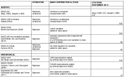
Table 2 compares and summarizes the di¤erent hybrid models, showing the estimation method, their

main contribution, and Google Scholar citations (November 2017 updated).

5.1

Additive Hybrid Models

The additive hybrid model augments the state-space model Equations (13) with a latent processzt:

1 2_{Originally, the composite likelihood is built combining marginal or conditional likelihoods of the true Data Generation}

Yt = 0( ) + 1( ) ~Zt+ zzt; (14)

~

Zt = T( ) ~Zt 1+R( ) t,

zt = 1zt 1+ t. (15)

The process zt is the measurement error represented by an autoregressive process. In such way, we …ll

the gap between the theory and the data relying on the dynamic structure of this error. There are several

examples of additive hybrid models: the DSGE-AR (Sargent, 1989, Altug, 1989), the DSGE-VAR à l’ Ireland

(2004), the DSGE-DFM (Boivin and Giannoni, 2006), the DSGE with non-modelled variables (Schorfheide,

Sill, and Kryshko, 2010), and the Augmented DSGE for Trends (Canova, 2014).

5.1.1 The DSGE-AR method

The …rst additive hybrid model was introduced by Sargent (1989) and Altug (1989). They propose to solve

DSGE model misspeci…cation by augmenting the model with (possibly serial correlated) unobservable errors

as described in Equation (14). This methodology combines the DSGE model with an AR model for the

measurement residuals.

In detail, a matrix 1 governs the persistence of the residuals; the covariance matrix, Et t 0t = V, is

uncorrelated. In this speci…cation the t’s generate the comovements between the observables, whereas the

elements ofztpick up idionsyncratic dynamics which are not explained by the structural part of the hybrid

model. However, if we set 0; 1 and z to zero, the DSGE model components can be used to describe the

‡uctuations ofYtaround a deterministic trend path, ignoring the common trend restrictions of the structural

model. For instance, Smets and Wouters (2003) estimate their model using this pattern with a two-step

procedure. In the …rst step, the deterministic trends are extracted from the data; in the second step, the

DSGE model is estimated using linear detrended observations.

Sargent (1989) and Altug (1989) assume that the measurement errors are uncorrelated with the data

generated by the model, hence the matrices 1andV are diagonal and the residuals are uncorrelated across

1 = 2 6 6 6 6 4

y 0 0

0 c 0

0 0 l

3 7 7 7 7 5 V = 2 6 6 6 6 4 v2

y 0 0

0 v2

c 0

0 0 v2l

3 7 7 7 7 5:

5.1.2 The DSGE-VAR à l’ Ireland

Ireland (2004) propose a general and multivariate framework for measurement errors, allowing the residuals

to follow an unconstrained, …rst-order vector autoregression. This approach has the main advantage of

imposing no restrictions on the cross-correlation of the measurement errors, allowing it to capture all the

movements and co-movements in the data not explained by the DSGE model. The matrices 1 and V are

given by: 1 = 2 6 6 6 6 4

y yc yl cy c cl ly lc l

3 7 7 7 7 5 V = 2 6 6 6 6 4 v2

y vyc vyl

vcy vc2 vcl

vly vlc vl2

3 7 7 7 7 5:

This framework is more ‡exible and general in the treatment of measurement errors, but some empirical

evidence (such as Fernández-de-Córdoba and Torres, 2011) shows the forecast performance of the traditional

DSGE-AR outperforms the DSGE-VAR à l’Ireland. Malley and Woitek (2010) propose an extension, allowing

for a vector autoregressive moving average (VARMA) process to describe the movements and co-movements

of the model’s errors not explained by the basic RBC model.

5.1.3 The DSGE-DFM

In macroeconomics, the researchers have access to large cross-sections of aggregate variables that include

measures of sectorial economic activities and prices as well as …nancial variables. Hybrid models can also be

these additional variables in the estimation potentially sharpens inference about latent state variables:

Yt = 0( ) + 1( ) ~Zt+zy;t; (16)

~

Zt = T( ) ~Zt 1+R( ) t, (17)

xt = 0+ 1t+ sst+zx;t; (18)

whereYtis the vector of the observable variables that are described by the DSGE model andxtis a large

vector of non-modelled variables.

Since the structure of this model resembles that of a dynamic factor model (DFM), e.g. Sargent and

Sims (1977), Geweke (1977), and Stock and Watson (1989), Schorfheide (2013) refers to the system (16) to

(18) as an example of a combination of DSGE and DFM (Boivin and Giannoni, 2006). Roughly speaking,

the vector of factors is given by the state variables associated with the DGSE model. The processeszy;tand

zx;tare uncorrelated across series and model idiosyncratic but potentially serially correlated movements (or

measurement errors) in the observables. Moreover, Equation (17) links the variablesxtto the DSGE model.

This relation generates comovements between theYt’ s and thext’ s and allows the computation of impulse

responses to the structural shocks t:

5.1.4 DSGE with non-modelled variables

Schorfheide, Sill, and Kryskho (2010) develop a method of generating a DSGE model-based forecast for

variables that do not explicitly appear in the model (non-core variables). They consider the following

representation:

Yt = 0( ) + 1( )&t; (19)

~

Zt = T( ) ~Zt 1+R( ) t;

where Eq (19) is the measurement equation, where&t= [ ~Zt0;Z~t0 1; Ms0( )]0 includes the state variables of

the model (Z~t), the lagged variables for the growth rates,Z~t0 1Ms0( )13. To this state-space representation,

we add an auxiliary regression:

1 3_{In Schorfheide, Sill, and Kryskho (2010), they assume the lagged values of output, consumption, investment, and real wages.}

zt= 0+cZ~t

0

jt s+ t;

where the cZ~t

0

jt is derived by the Kalman Filter to obtain estimates of the latent state variables, based

on the DSGE model parameter estimates. t is a variable-speci…c noise process, t = t 1 + t and t N(0; 2):

This augmented state-space can be interpreted as a factor model. The factors are given by the state

variables of the DSGE model, while the measurement equation associated with the DSGE model describes

the way in which the core macroeconomic variables load on factors, and the auxiliary regression describes

the way in which additional (non-core) macroeconomic variables load on the factors. This representation

is a simpli…ed version of the DSGE-DFM since the DSGE with non-modelled variables do not attempt to

estimate the DSGE model and the auxiliary regression simultaneously.

5.1.5 The Augmented DSGE for Trends

One of the most discussed problem in using a DSGE model for estimation is its inability to capture the

long-run features of the data. Canova (2014) proposes a way to correct these problems using the following

hybrid model:

Yt = 0( ) + 1( ) ~Zt+ zzt (20)

~

Zt = T( ) ~Zt 1+R( ) t;

zt = 1zt 1+ 2zt 1+ t;

zt = zt 1+vt:

Depending on the restrictions imposed on the variances of tand t, the processztis integrated of order

one or two and can generate a variety of stochastic trend dynamics.

5.2

Hierarchical Hybrid Models

The second class of hybrid models used for estimating the DSGE model is the hierarchical hybrid.

Yt = 0( ) + 1( ) ~Zt+vt; (21)

~

Zt = 1( ) ~Zt 1+ ( ) t;

where

i = i( ) + i ; i= 0;1 (22) i = i( ) + i ; i= 1; :

In this setup, i( )and i( )are interpreted as restrictions on the unrestricted state-space matrices i

and i; instead, the disturbances, i and i can capture deviations from the restriction functions i( )and i( ). This kind of hybrid model is related to Bayesian econometrics, since the stochastic restrictions (22)

correspond to a prior distribution of the unrestricted state-space matrices conditional on the DSGE model

parameters :

In the literature, there are three examples of hierarchical hybrid models: the DSGE-VAR (Del Negro

and Schorfheide, 2004), the DSGE-FAVAR (Consolo, Favero, and Paccagnini, 2009), and the Augmented

(B)VAR (Fernández-de-Córdoba and Torres, 2011).

5.2.1 The DSGE-VAR

Based on the work of Ingram and Whiteman (1994), the DSGE-VAR approach proposed by Del Negro and

Schorfheide (2004) uses the DSGE model to generate prior distributions for the VAR. The starting point for

the estimation is the unrestricted VAR of orderp:

Y_{t= 0+ 1}Y_{t 1+:::+ p}Y_{t p+}u_{t. (23)}

The companion form is:

Y =X +U; (24)

Y is a(T n)matrix with rowsY0

t; X is a(T k)matrix(k= 1 +np; p=number of lags)with rows

X0

t= [1; Yt0 1; :::; Yt p0 ], U is a (T n)matrix with rowsu0t and is a (k n) = [ 0; 1;:::; p]0:

past observations of Y:

The log-likelihood function of the data is written as a function of and u:

L(Yj ; u)/ j uj

T

2 exp 1

2tr

1

u (Y0Y 0X0Y Y0X + 0X0X ) : (25)

Meanwhile, the prior distribution for the VAR parameters proposed by Del Negro and Schorfheide (2004)

is based on the statistical representation of the DSGE model given by the VAR approximation.

Let xx; yy; xy and yxbe the theoretical second-order moments of the variablesY andX implied by

the DSGE model, where:

( ) = xx1( ) xy( ) (26)

( ) = yy( ) yx( ) xx1( ) xy( ):

The moments are the "dummy observation priors" (Theil and Goldberg, 1961, and Ingram and Whiteman,

1994) implemented in the hybrid model. These vectors can be interpreted as the probability limits of the

coe¢cients in a VAR estimated on the arti…cial observations generated by the DSGE model.

Conditional on the vector of structural parameters in the DSGE model , the prior distributions for the

VAR parametersp( ; uj )are of the Inverse-Wishart (IW) and Normal forms:

uj IW(( T u( ); T k; n) (27)

j u; N ( ); u ( T XX( )) 1 ;

where the parameter controls the degree of model misspeci…cation with respect to the VAR: for small

values of the discrepancy between the VAR and the DSGE-VAR is large and a sizeable distance is generated

between the unrestricted VAR and DSGE estimators. On the contrary, large values of correspond to small

model misspeci…cation and for =1beliefs about DSGE misspeci…cation degenerate to a point mass at

zero. Bayesian estimation could be interpreted as estimation based on a sample in which data are augmented

by a hypothetical sample in which observations are generated by the DSGE model, the "dummy observation

priors". Within this framework, determines the length of the hypothetical sample.

The posterior distributions of the VAR parameters have also the Inverse-Wishart and Normal forms.

uj ; Y IW ( + 1)T

^

u;b( );( + 1)T k; n (28)

j u; ; Y N

^

b( ); u [ T XX( ) +X0X] 1 (29)

^

b( ) = ( T XX( ) +X0X) 1( T XY( ) +X0Y)

^

u;b( ) =

1

( + 1)T ( T Y Y( ) +Y

0_{Y) ( T}

XY( ) +X0Y)

^

b( ) ;

where the matrices ^b( )and

^

u;b( )have the interpretation of maximum likelihood estimates of the VAR

parameters based on the combined sample of actual observations and arti…cial observations generated by the

DSGE. Equations (28) and (29) show that the smaller is;the closer the estimates are to the OLS estimates of an unrestricted VAR. Instead, the higher is, the closer the VAR estimates will be tilted towards the

parameters in the VAR approximation of the DSGE model (^b( )and

^

u;b( )).

To obtain a non-degenerate prior density (27), which is a necessary condition for the existence of a

well-de…ned Inverse-Wishart distribution and for computing meaningful marginal likelihoods, has to be

greater than M IN, such that: M IN n+_Tk;k= 1 +p n, wherep=lags and n=endogenous variables.

Consequently, the optimal lambda must be greater than or equal to the minimum lambda b M IN .

The DSGE-VAR tool allows the researcher to draw posterior inferences about the DSGE model

pa-rameters : Del Negro and Schorfheide (2004) provide evidence that the posterior estimate of has the interpretation of a minimum-distance estimator, where the discrepancy between the OLS estimates of the

unrestricted VAR parameters and the VAR representation of the DSGE model is a sort of distance

func-tion. The estimated posterior of parameter vector depends on the hyperparameter . When ! 0, in

the posterior the parameters are not informative, so the DSGE model is of no use in explaining the data.

Unfortunately, the posteriors (29) and (28) do not have a closed form and we need a numerical method to

solve the problem. The posterior simulator used by Del Negro and Schorfheide (2004) is the Markov Chain

Monte Carlo Method and the implemented algorithm is the Metropolis-Hastings acceptance method. This

procedure generates a Markov Chain from the posterior distribution of and this Markov Chain is used for

Monte Carlo simulations. See Del Negro and Schorfheide (2004) for more details.

The optimal is given by maximizing the log of the marginal data density:

b= arg max

> M I N

lnp(Yj ):

model is called DSGE-VAR b andbis the weight of the priors. It can also be interpreted as the restriction

of the theoretical model on the actual data.

Unfortunately, Del Negro and Schorfheide (2004) do not propose any statistical tool to verify the power

of their procedure. Moreover, Del Negro, Schorfheide, Smets and Wouters (2007b) explain "...the goal of

our article is not to develop a classical test of the hypothesis that the DSGE model restrictions are satis…ed;

instead, we stress the Bayesian interpretation of the marginal likelihood function of p( jY), which does not require any cuto¤ or critical values. ... ".

Several recent papers apply the DSGE-VAR to detect possible misspeci…cations in DSGE models and

evidence how this econometric tool is a useful forecasting combination model which improves the prediction

ability of DSGE model with the powerful time series analysis through VAR (see Adolfson, Laséen, Lindé, and

Villani, 2008; Ghent, 2009; Kolasa, Rubaszek, and Skryzpczynski, 2012; Consolo, Favero, and Paccagnini,

2009; Lees, Matheson and Smith, 2011; Bekiros and Paccagnini, 2013, 2014, 2015, and 2016; Gupta and

Steinbach, 2013; Bhattacharjee and Gelain, 2017, among others).

5.2.2 The DSGE-FAVAR

In the DSGE-FAVAR (Consolo, Favero, and Paccagnini, 2009), the statistical representation is a Factor

Augmented VAR instead of a VAR model. A FAVAR benchmark for the evaluation of the previous DSGE

model will take the following speci…cation:

0 B @ Y_t F_t 1 C A= 2 6

4 11(L) 12(L)

21(L) 22(L)

3 7 5 0 B @

Y_{t 1} F_{t 1}

1 C A+ 0 B @ uZ t uF t 1 C

A; (30)

whereYtare the observable variables included in the DSGE model andFtis a small vector of unobserved

factors extracted from a large data-set of macroeconomic time series, which capture additional economic

information relevant to modelling the dynamics of Yt. The system reduces to the standard VAR used to

evaluate DSGE models if 12(L) = 0:

Importantly, and di¤erently from Boivin and Giannoni (2006), the FAVAR is not interpreted as the

reduced form of a DSGE model. In fact, in this case the restrictions implied by the DSGE model on a

general FAVAR are very di¢cult to trace and model evaluation becomes even more di¢cult to implement. A

very tightly parameterized theory model can have a very highly parameterized reduced form if one is prepared

to accept that the relevant theoretical concepts in the model are a combination of many macroeconomic and

5.2.3 The Augmented (B)VAR

The Augmented (B)VAR (Fernández-de-Córdoba and Torres, 2011) is a combination of the unrestricted

VAR with the DSGE model and is conducted by increasing the size of the VAR representation. In this

methodology, xt is a vector of observable economic variables assumed to drive the dynamics of the

econ-omy. The structural approach assumes that DSGE models contain additional economic information, not

fully captured by xt. The additional information is summarized by using a vector of unobserved variables

zt. Fernández-de-Córdoba and Torres (2011) explain that these non-observed variables can be total factor

productivity, marginal productivity, or any other information given by the economic model, but they do not

belong to the observed variable set.

The joint dynamics of (xt; zt) are given by the following transition equation:

2 6 4 xt

zt

3 7

5= (L)

2 6 4 xt 1

zt 1

3 7 5+ 2 6 4 " x t "z t 3 7 5:

This system cannot be estimated directly since zt are non-observed, but zt can be obtained using the

DSGE model to create a new variable Zt, which is used to expand the size of the VAR. It is possible to

construct a VAR with the following speci…cation:

2 6 4 xt

Zt 3 7 5= 2 6

4 11(L) 12(L)

21(L) 22(L)

3 7 5

2 6 4 xt 1

Zt 1

3 7 5+ 2 6 4 " x t "z t 3 7 5;

where xt are the macroeconomic data that the DSGE model seeks to explain andZtis a vector derived

from the DSGE model. If the model speci…cation is correct, the relation between xt and Zt should then

capture additional economic information relevant to modelling the dynamics ofxt. A standard unrestricted

ESTIMATION MAIN CONTRIBUTION for DSGE CITATIONS (NOVEMBER 2017) ADDITIVE

DSGE-AR

Altug (1989), Sargent (1989)

Maximum Likelihood

Introduce a univariate

measurement (AR) Altug (1989): 321; Sargent (1989):

419

DSGE-VAR à l'Ireland Ireland (2004)

Maximum Likelihood

Introduce a multivariate measurement (VAR)

502

DSGE-DFM

Boivin and Giannoni (2006) Bayesian Latent variables

added to state-space

263

DSGE with non-modelled variables Schorfheide, Sill, and Kryshko (2010)

Bayesian

Auxiliary regressions like measurement equations

in a DFM linking non-core variables to

state-space of DSGE 56

DSGE for trends Canova (2012)

Maximum Likelihood Bayesian

De-trend equation for variables added to state space

40

HIERARCHICAL

DSGE-VAR

Del Negro and Schorfheide (2004) Bayesian

VAR representation added

by artificial data from DSGE ₅₄₃

DSGE-FAVAR

Consolo, Favero, and Paccagnini (2009)

Bayesian FAVAR representation added_{by artificial data from DSGE}

47 Augmented (B) VAR

Fernandéz-de-Cordoba and Torres (2011)

Bayesian Non-observed variables_{from DSGE added to state space}

12

Table 2: Comparison

6

Concluding Remarks

Dynamic Stochastic General Equilibrium (DSGE) models are the main tool used in Academia and in Central

Banks to evaluate the business cycle for policy and forecasting analyses. Despite the recent advances in

improving the …t of DSGE models to the data, misspeci…cation issue still remains. This survey shed light

on the sources and the remedies to face with misspeci…ed DSGE models. We distinguish four forms of

misspeci…cation: a) Misspeci…cation in the State-Space Representation, b) Misspeci…cation in Parameters, c)

Misspeci…cation in the Assumptions of the DSGE model, and d) Misspeci…cation in Computational Methods.

We discuss several attempts to identify the sources of misspeci…cation, in particular about the State-Space

representation, such as Monti (2015) and Inonue, Kuo, and Rossi (2017). Meanwhile, Canova and Matthes

(2017) and Den Haan and Dreschel (2017) contribute to the literature proposing two di¤erent methodologies

which are not only able to detect the sources but they aim to reduce the degree of misspeci…cation.

In addition, Additive Hybrid and Hierarchical Hybrid models are illustrated as remedies to face with

References

[1] Adolfson, Malin, Stefan Laséen, Jesper Lindé, and Mattias Villani (2008): "Evaluating an Estimated

New Keynesian Small Open Economy Model", Journal of Economic Dynamics and Control

Else-vier, vol. 32(8), pages 2690-2721.

[2] Albonico, Alice, Alessia Paccagnini, and Patrizio Tirelli (2016): "In Search of the Euro-Area Fiscal

Stance",Journal of Empirical Economics, Elsevier, vol. 39(PB), pages 254-264.

[3] Albonico, Alice, Alessia Paccagnini, and Patrizio Tirelli (2017): "Great Recession, Slow Recovery, and

Muted Fiscal Policies in the US",Journal of Economic Dynamics and Control, Elsevier, vol. 81(C),

pages 140-161.

[4] Alessi, Lucia, Matteo Barigozzi, and Marco Capasso (2011): "Nonfundamentalness in structural

econo-metric models: a review",International Statistical Review, 79 (1). 16-47. ISSN 0306-7734.

[5] Altug, Sumro (1989): "Time-to-Build and Aggregate Fluctuations: Some New Evidence",International

Economic Review, 30(4), pp. 889-920.

[6] An, Sungbae and Frank Schorfheide (2007): "Bayesian Analysis of DSGE Models",Econometric

Re-views, Taylor and Francis Journals, vol. 26(2-4), pages 113-172.

[7] Angelini, Giovanni and Luca Fanelli (2016): "Misspeci…cation and Expectations Correction in New

Keynesian DSGE Models",Oxford Bulletin of Economics and Statistics, 78 (5), 623-649.

[8] Aruoba, Boragan, Luigi Bocola, and Frank Schorfheide (2017): "Assessing DSGE model

nonlineari-ties",Journal of Economic Dynamics and Control, Volume 83, October, Pages 34-54.

[9] Bhattacharjee, Arnab and Paolo Gelain (2017): " How much does the FOMC care about model

misspeci…cation?", Manuscript.

[10] Basu, Susanto and Brent Bundick (2017): "Uncertainty Shocks in a Model of E¤ective Demand",

Econometrica, Volume 85, Issue 3, May, Pages 937–958.

[11] Beaudry, Paul, Patrick Fève, Alain Guay, and Franck Portier (2015): "When is nonfundamentalness

in VAR a real problem? An application to news shocks", NBER Working Paper No. 21466.

[12] Bekiros, Stelios and Alessia Paccagnini (2013): "On the Predictability of Time-Varying VAR and

DSGE Models",Empirical Economics, Springer, vol. 45(1), pages 635-664, August.

[13] Bekiros, Stelios and Alessia Paccagnini (2014): "Bayesian Forecasting with a Small and Medium

Scale Factor-Augmented Vector Autoregressive DSGE Model", Computational Statistics & Data