Underspecified Semantic Representation
Mehdi Manshadi
∗ University of RochesterDaniel Gildea
∗∗ University of RochesterJames F. Allen
† University of RochesterThe general problem of finding satisfying solutions to constraint-based underspecified represen-tations of quantifier scope is NP-complete. Existing frameworks, including Dominance Graphs, Minimal Recursion Semantics, and Hole Semantics, have struggled to balance expressivity and tractability in order to cover real natural language sentences with efficient algorithms. We address this trade-off with a general principle of coherence, which requires that every variable introduced in the domain of discourse must contribute to the overall semantics of the sentence. We show that every underspecified representation meeting this criterion can be efficiently pro-cessed, and that our set of representations subsumes all previously identified tractable sets.
1. Introduction
Quantifier scope ambiguity is a big challenge in deep language understanding systems. Consider the following conversation:
Woman:I believe there is one true soulmate for every person.
Man:He must be very busy.1
Most people find the man’s answer unusual (humorous, sarcastic, etc.). This is because one of the two scopings of the woman’s sentence feels so obvious that the less likely
∗Department of Computer Science, University of Rochester, Rochester, NY 14627. E-mail:[email protected].
∗∗Department of Computer Science, University of Rochester, Rochester, NY 14627. E-mail:[email protected].
†Department of Computer Science, University of Rochester, Rochester, NY 14627. E-mail:[email protected].
1dilbert.com/strip/2001-04-19.
Submission received: 2 June 2016; revised version received: 13 March 2017; accepted for publication: 1 August 2017.
scoping is often missed at first glance. In the most likely interpretation, where there are many soulmates, the quantifiereveryhaswide scope, and, in the second interpretation, where there is a unique soulmate,everyhasnarrow scope. The following conversation is of a similar nature:
Bob:How long have you and Opal been married now Earl?
Earl:I’ve lost track. But I can tell you this ... I don’t regret one day of it.
Bob:Which day don’t you regret?2
The difference, however, is that, in this example, the scope ambiguity is not be-tween two quantifiers, but bebe-tween a quantifier (one) and a scopal operator (negation). Underspecification, that is, generating an unscoped semantic representation, has been the most common way of dealing with quantifier scope ambiguity since the early days of natural language processing. Underspecification is not adopted only because quan-tifier scope disambiguation is difficult, but also because, for most practical purposes, an underspecified representation (UR)3 will do the job. Equations (1) and (2) show an
unscoped logical form (LF) for the sentencesThere is one soulmate for every personand I do not regret one day, respectively.
hOne x Soulmatei hEvery y Personi
Of(x, y)
(1) h
One x Dayi
Not(Regret(I, x)) (2)
Equation (3) shows the two scopings of the unscoped LF in Equation (2):
One(x,Day(x),Not(Regret(I,x)))
Not(One(x,Day(x),Regret(I,x))) (3)
When the number of quantifiers increases, the number of possible scopings will increase exponentially. More recent underspecification formalisms are constraint-based—that is, they allow for constraints, restricting the order of quantifiers, to be added to filter out unwanted scopings. The constraints can come from different sources, including deeper processing steps, such as discourse or pragmatics. Several constraint-based underspec-ification frameworks have been developed over the past couple of decades. Minimal Recursion Semantics (MRS) (Copestake, Lascarides, and Flickinger 2001), Hole Seman-tics (Bos 2002), and Dominance Constraints (Koller, Niehren, and Thater 2003) are among those frameworks. Each framework is different in the type of constraints it allows, and has its own advantages and disadvantages. A constraint-based UR defines
2 FromPickles(Brian Crane, 2005).
a computational problem that needs to be solved: Given a UR with a set of constraints, one needs to check if these constraints are consistent, that is, whether there is a scoping satisfying all the constraints. This is called thesatisfiabilityproblem. The satisfiability problem for all these three frameworks, in their general form, is intractable (Althaus et al. 2003). There has been some effort towards defining a notion ofwell-formedness within the context of these frameworks. The goal has been to define a subset of URs, the so-called well-formed UR, for which the satisfiability problem becomes tractable. For ex-ample, Niehren and Thater (2003) defined the notion of (weak) net to characterize such a subset. Well-formedness was also intended to bridge the gap between these under-specification formalisms; the hope was that the differences between these formalisms disappear and they become equivalent once restricted to well-formed structures.
As seen in Niehren and Thater (2003) and Fuchss et al. (2004), the problem with those efforts on defining a notion of well-formedness is that their satisfaction of both properties was only empirically supported, and hence the correctness of those state-ments has remained a conjecture. In better words, first, there was no mathematical proof to show that nets enforce the equivalence of qeq vs. dominance relations, the two dif-ferent types of constraint used in MRS vs. Dominance Constraints/Hole Semantics, and second, although they were proved to be tractable, there was no convincing linguistic justification as to why nets cover all URs corresponding to coherent sentences. In fact, this claim was later falsified when Thater (2007) presented examples of coherent sen-tences that were unaccounted for by nets (Section 7.1). In summary, it has remained an open question whether there is a linguistically justified notion of well-formedness that not only (provably) bridges the gap between the above formalisms, but also guarantees tractability. In this article, we propose such a notion of semantic coherence that not only answers both of these open questions but also solves several other unanswered questions within the context of scope underspecification. The contribution of this work can be summarized as follows:
r
We extend the previous tractable frameworks to cover those naturallanguage sentences that were known to be unaccounted for without increasing the complexity of the algorithms.
r
We go beyond those known unaccounted examples and, once andfor all, prove that every semantically coherent natural language sentence (based on a linguistically justified notion of semantic coherence) can be solved in polynomial time, presenting a definitive answer to the open question of whether solving unscoped representations of real-life natural language sentences within the context of these formalisms is
tractable.
r
We prove that, under our notion of coherence, the two fundamentallydifferent types of constraint, dominance and qeq, become equivalent, hence, the principal difference between these formalisms disappears.
r
We further bridge the gap between the constraint-based formalisms bylabel-to-label dominance relations in nature, can be represented by hole-to-label dominance relations, as long as the URs are coherent. This explains how a formalism such as Hole Semantics, which does not incorporate label-to-label dominance relations, does not lack the power to model binding constraints.
r
Finally, given that quantifier scoping has traditionally been treated as anordering problem (i.e., predicting a permutation of quantifiers), whereas in the constraint-based formalisms it is defined as predicting a tree structure, our notion of coherence allows us to explain this discrepancy. We show that, for coherent URs, quantifier scoping is reduced from predicting a tree structure to finding a permutation.
Whereas we focus on finding solutions to underspecified representations with hard constraints, our results have implications for statistical systems based on soft con-straints. Because weighted soft constraints generalize hard constraints, finding efficient algorithms for solving systems with hard constraints is a first step toward finding efficient algorithms for finding the highest-scoring solution under weighted constraints. We also show how our algorithm for finding solutions under hard constraints can be used to guide search for the highest scoring solution given a combination of hard and soft constraints.
Some of this article’s results (or a weaker version of them) have been proved in our own previous work. In Manshadi, Allen, and Swift (2008b), we proved the equiv-alence of qeq and dominance for canonical form MRS, which motivated the notion of completeness. In Manshadi, Allen, and Swift (2009), we introduced the notion of heart-connectedness, which, in the current work, forms the basis of coherence. In another line of work (Manshadi and Allen 2012), we introduced a superset of nets, called supernets, that covered the known examples unaccounted for by nets.
Coherent UG Section 4 Dominance Graph
Coherent MRS (satisfiable and heart-connected)
Section 7.2 MRS
Normal DG
Hole Semantics’s UR
(satisfiable and hyper-normally connected) Section 7.3
Hypernet Section 5
Weak net Section 7.1 Weakly Normal DG
Underspecification Graph Section 2
CF-MRS Complete UG
[image:5.486.54.435.62.363.2]Section 3
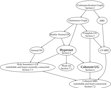
Figure 1
Classes of underspecification graph introduced in this article. We define hypernet, show that it is computationally tractable, and further show that it covers all coherent sentences, and that it subsumes previously identified tractable classes.
give a formal definition of our universal framework (i.e., underspecification graph). Section 3 defines a notion of completeness and proves that, under this notion, the two fundamentally different types of constraint used in underspecification formalisms (qeq and dominance) become equivalent. Section 4 defines a notion of coherence for a complete UR. Section 5 discusses the tractability issue. We propose a tractable subset of URs and prove that it is the largest tractable subset found so far. We then show that every coherent UR belongs to this set, and we discuss implications for systems of mixed hard and soft constraints. Section 6 shows that scope disambiguation can be treated as an ordering problem. Finally, Section 7 gives a detailed comparison of our framework with previous work, and Section 8 concludes.
2. Underspecification Graph
Consider the following example.
Early systems (Schubert and Pelletier 1982; Hobbs and Shieber 1987; Allen 1995) repre-sented the semantics of such a sentence using an unscoped LF of the following general form:
Every(x,Child(x,y),), A(y,Politician(y),), Run(x) (4)
To scope this LF, at each step, a quantifier is picked and the main predication (i.e., Run(x)) or the partially scoped formula built so far is fused to its body hole:
Step 1. Every(x,Child(x,y),Run(x))
Step 2. A(y,Politician(y),Every(x,Child(x,y),Run(x))) (5)
By picking quantifiers in different orders, different scopings are generated.
Next, the notion of constraints was introduced into the domain of scope underspeci-fied semantics. For example, Quasi Logical Form (Alshawi and Crouch 1992) allows for constraints such asA>Everyto be used to force one quantifier to rest within the scope of another. By inventing some machinery that allows for Discourse Representation Theory (Kamp 1981) to support scope underspecification, Underspecified Discourse Representation Theory (or UDRT) (Reyle 1993) takes the notion of constraint-based underspecification to a new level. UDRT introduces a complex system of constraints, that, among other things, can define a maximum and a minimum range for the scope of a quantifier relative to other scope bearing elements. It is fair to say that Reyle’s work inspired the next two decades of research on constraint-based scope underspecification, resulting in several underspecification formalisms such as Hole Semantics (HS; Bos 1996), MRS (Copestake, Lascarides, and Flickinger 2001), and Dominance Graph (DG; Thater 2007). Unlike Quasi Logical Form or UDRT, the new formalisms treat underspec-ification as an abstract algebraic framework which is independent of the target object language, whether it is first order predicate calculus, modal logic, Discourse Represen-tation Theory, etc. A UR in these formalisms is a set of abstract labeled formulas with holes that can be filled in with other labeled formulas. The formulas come with a set of constraints between the labels and holes, and in order for a scoping to be considered valid, the set of constraints ought to be respected. Despite all the similarities, as will be seen shortly, HS/DG and MRS differ in how they interpret the constraints.
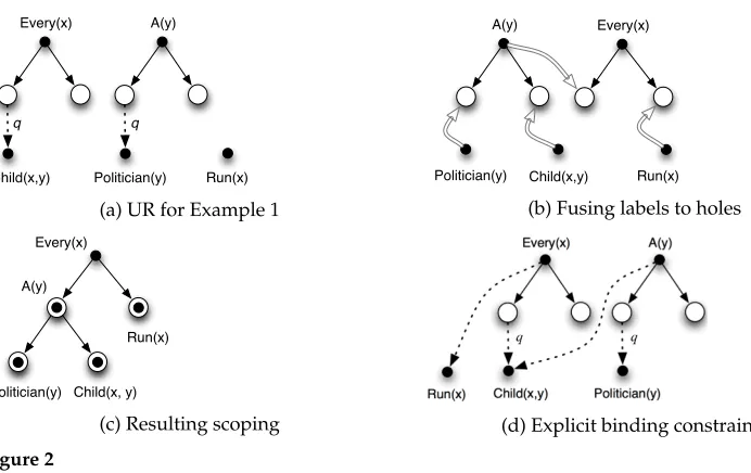
Figure 2 shows the graphical depiction of the UR of Example (1) as proposed by MRS. Solid nodes represent labeled formulas, and are called label nodes. The holes of the formulas are represented by nodes with hollow circles, called thehole nodes. Scopings of such a structure are built by fusing label nodes to hole nodes as shown in Figure 2(b). This UR leaves both the body and the restriction of the quantifiers underspecified. This is to allow for scopings such as Figure 2(c), in which quantifierA lies between quantifierEveryand its restriction. The dotted line between the label node Child(x,y), call itl, and the restriction hole ofEvery, call ith, is an example of a constraint. This constraint (also represented ash=ql), requires that eitherhis directly filled bylor
Politician(y) A(y)
Child(x,y) Every(x)
Run(x)
q q
(a) UR for Example 1
Politician(y) A(y)
Child(x,y) Every(x)
Run(x)
(b) Fusing labels to holes
Every(x)
A(y)
Politician(y)
Run(x)
Child(x, y)
[image:7.486.62.408.58.276.2](c) Resulting scoping (d) Explicit binding constraints
Figure 2
Using graphical notation to represent unscoped LF.
to see that qeq directly implements the idea of wrapping a quantifier around a formula as shown in Equation (5). It is easy to see that not every assignment of labels to holes in the UR is a valid scoping, even if it satisfies both qeq constraints. This is because, in addition to qeq constraints, the UR carries a group of implicit constraints, the so-called binding constraints. The binding constraints force every variable (x,y, etc.) to be in the scope of its quantifier. Unlike qeq, binding constraints enforce a mere outscoping (a.k.a. dominance) relation. That is, to satisfy a binding constraint fromutov, it is enough that uoutscopes (a.k.a. dominates)v.
To simplify things, let us make the binding constraints explicit by using unlabeled dotted edges as shown in Figure 2(d). We call the resulting representation that incor-porates both dominance and qeq constraints an underspecification graph (UG).
Before moving to the formal definition of UG, it should be emphasized that what is defined here as UG is nothing but the integration of the three existing concepts: MRS, HS, and DG. Defining a framework that subsumes all three has proved very useful in substantiating the results we have obtained and in providing rigorous proofs. Otherwise, from a practical standpoint (as proved later), UG has little to no advantage over DG. In addition, it serves us better to first define the general framework, and then introduce subsets of it, rather than the other way around.
2.1 The Formal Definition
l l
h1 hn
(a) General form of ET
q q
l2 l4
l3 l5
h1 h2 h3 h4
q
l0
l1 h0
[image:8.486.58.379.60.167.2](b) An example of UG
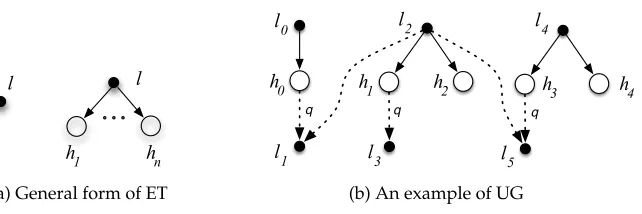
Figure 3
Elementary tree and underspecification graph.
Definition 1 (Elementary Tree)
Anelementary treeorET(a.k.a. fragment) is anordered4tree of depth 0 or 1. Theroots of all ETs are represented by small solid circles and are referred to as label nodesor simplylabels. All the leaf nodes of the ETs of depth 1 are represented as big hollow circles and are referred to as hole nodes or simplyholes. ETs with holes are called scopal ETs.5
Figure 3(a) shows the general form of an elementary tree for both cases ofdepth=0 anddepth=1. Whendepth=0, the elementary tree is asingleton.
Definition 2 (Underspecification Graph)
The 8-tupleU=hLU,HU,EU,QU,DU,TU,LqU,PUiis called a (scope)Underspecification
Graphor in shortUG, if it is a finite structure with the following properties:
r
FU=hLU,HU,EU,PUiis a forest of elementary trees, withLUbeing the setof label nodes,HUthe set of hole nodes, andEUthe set of directed solid
edges, going from the root of ETs to their holes. The order of holes in each ET is defined byPU.6In graphical notation,PUis not explicitly given, as it
is implicit in the left-to-right order by which the hole nodes of each ET are depicted.
r
QUis a relation fromHUtoLU, that is,QU ⊂HU×LU. In graphicalnotation, each (h,l)∈QUis represented as a directeddottededge fromhto
lmarked with a labelq, called aqeq constraint.
4 Throughout this paper, unless otherwise specified, by tree we always mean a rooted ordered tree. 5 A mathematically precise definition requires ETs to be defined as graphs over pairs (u,s), whereuis a
node andsis a symbol of the valueL(for label nodes) orH(for hole nodes). Such notation will be quite cumbersome and may become confusing, especially given that we later need to define two types of edges, and even two types of dotted edges. Therefore, although we understand that the underlying mathematical model is defined in this precise way, we avoid adopting the notation. Instead, we usel,l1, and so forth, to denote labels andh,h1, and so forth, to denote holes. The same applies to different types of edges defined later.
r
DUis a relation overHU∪LU. Each (u,v)∈DUis called adominance constraintand, in graphical notation, is represented as a directed dottededge from nodeuto nodev. The dominance constraints can go from any node to any node, except from holes to holes, therefore,DU⊂(LU∪HU)×(LU∪HU)−HU×HU. Dominance (as opposed to qeq) is the
default constraint type, therefore, the labeldis dropped for the sake of brevity.
r
TU is a dummy ET of depth 1, withl0∈LU,h0∈HU, ande0=(l0,h0)∈EUbeing its root, its single hole, and its single edge. It is defined to be the designated root of every scoping, therefore,TU,l0, andh0are calledtop
ET,top label, andtop hole, respectively.7The set of all labels exceptl 0is
denoted by ˜LU, that is, ˜LU =def LU− {l0}.
r
LqU⊂L˜Uis the set offloating scopal nodes. The ETs rooted at these nodes
are calledfloating scopal ETs. Every scopal ET other than the floating scopal ETs is called afixed-scopal ET. Floating scopal ETs are required to have a hole as the right-most child of the root. This hole and its connecting edge (sometimes distinguished with a label “b” for emphasis) are called the body hole, and the body edge, respectively. In practice, floating scopal ETs correspond to (generalized) quantifiers. Therefore, we use the terms floating-scopaland(generalized) quantifierinterchangeably. Quite often, we do not explicitly defineLqU, because (generalized) quantifiers can be recognized from the context. Because quantifiers have one restriction and one body preposition, throughout this article we only consider floating scopals with two holes.
Scopings of a UG are built by fusing labels to holes. We call this afusion.8
Definition 3 (Fusion)
Given a UGU, a (total)fusionf is a total function from ˜LUtoHU. A partialfusionf is a
partial function from ˜LUtoHU.
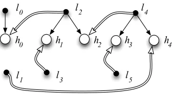
Figure 4(a) demonstrates a fusion for the UG Uin Figure 3(b). Given a fusion f, the corresponding scoping is denoted byTU,f. We construct the graph ofTU,f fromU
by removing all the constraint edges and fusingltof(l) for eachl∈L˜U, as illustrated in
7 Most underspecification frameworks, such as MRS or Hole Semantics, implement such an ET, which does not correspond to an actual predication of the sentence, but serves as the highest level predication of the sentence, encompassing the overall semantics. For example, in a typed feature structure formalism like MRS, this ET contains attribute-value pairs, encoding some global semantic properties of the sentence, such as the speech act, which is not particular to any individual elementary predication.
l2
l0 l4
l3 l5
h1 h2
h0 h3 h4
l1
(a) Graphical depiction of a fusion function
l0
l3
(
,
h)1
l5
(
,
h3) (l1,
h4)l
4
(
,
h2)l2
(
,
h0) [image:10.486.290.386.61.183.2] [image:10.486.56.224.87.179.2](b)TU,ffor fusionfon left Figure 4
Building a solution for a UG.
Figure 4(b). Intuitively, we expect scopings to form a tree. Theorem 1 states the necessary and sufficient condition forTU,f to be a tree.
Theorem 1
Given a UGUand a total fusionf ofU,TU,fis a rooted tree if and only ifTU,f is acyclic.
Proof.The “only if” direction is trivial. The “if” direction holds for the following reason. Becausefis a function, every label is fused into at most one hole, hence, has at most one parent inTU,f. Iff is total, then every label exceptl0is fused into exactly one hole, hence,
has exactly one parent inTU,f. Therefore, withUbeing finite, if we start at any arbitrary
node and follow the sequence of parents, we have to end up atl0. This meansTU,f is a
tree rooted atl0. 2
Although fusion is defined as any function from ˜LtoH, we are only interested in fusions that result in valid readings, that is, satisfy the constraints.
Definition 4 (Constraint Satisfaction and Admissibility) Fusionf (similarlyTU,f)satisfies
r
a qeq constraintq=(h,l), ifh=f(l), or the directed path fromhtolin TU,f9consists of only the body edges of quantifier ETs (called ab-path);r
a dominance constraintd=(u,v), ifudominatesvinTU,f.Fusionf ofUisadmissibleifTU,f is acyclic and satisfies all the constraints inU.
So far we have informally used the term scoping to refer to a fully scope-disambiguated UR. We now formally define this notion and call it a solution.
Definition 5 (Solution)
T is called asolutionof a UGUiffT =TU,ffor some admissible, total, andonto10fusion
fofU. In informal contexts, solutions are sometimes referred to asreadings.Uis called satisfiableifUhas at least one solution.
In this definition, admissibility ensures the satisfaction of all constraints, totality ensures that every label (except the top) is fused into some hole, and onto-ness ensures that no hole is left unfused. Following Lemma 1, Definition 5 guarantees that every solution is a tree structure. The fusion in Figure 4(a) is admissible, total, and onto, and hence, Figure 4(b) is a solution.
The following definition will later be used for the comparison of our framework with other frameworks.
Definition 6 (Merging-Free Solutions)
The solutionTU,f is called amerging-free, iff is a one-to-one function. Otherwise, it is
called a merging solution.
The following lemma directly follows from the definition.
Lemma 1
Given a UGUand a solutionT ofU,T is merging-free if and only if|L˜U|=|HU|.
Corollary 1
Either all the solutions of a UG are merging-free or none are.
In practice, merging solutions only happen when the underspecified representation is incomplete, that is, when there are ETs that are floating around and, in order to build a solution, they must be fixed up with other ETs to make conjunctions. In Section 3, we prove that all solutions of a complete UG are merging-free.
2.2 Variations of UG
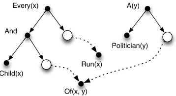
The definition of UG requires each ET to be of depth at most one and, when the depth is exactly one, all the leaf nodes to be hole nodes. This definition perfectly imitates the notion of elementary predications in MRS, but some frameworks, such as Hole Semantics, use the concept of (labeled) formula, which does not precisely fit into this definition. Figure 5(a) shows a graph, roughly corresponding to the UR that Hole Semantics assigns to the sentenceEvery child of a politician runs. As seen in this figure, we have to deal with ETs with depth more than one and leaves that are not necessarily a hole. Even in MRS, ETs can be stacked to form trees of depth more than one. Figure 5(b)
Every(x)
Child(x)
Run(x)
A(y)
Politician(y)
Of(x, y) And
(a) Hole Semantics UR with stacked ET
Cat(y) A(y)
Dog(x) Every(x)
Chase(x, y)
q q
Bark(x) And
[image:12.486.47.226.63.161.2](b) MRS structure for the sentence in Example (2)
Figure 5
Examples of stacked ETs.
shows the MRS structure of the following sentence in graphical notation, obtained from English Resource Grammar.11
2. Every dog barks and chases a cat.
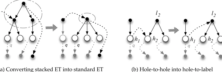
Finally, a partially scoped UGU, even if all the ETs ofUare standard, will inevitably have these non-standard tree structures. Therefore, for the sake of the robustness of our definitions, we should be able to model these structures. Fortunately, we will be able to do this without too much effort. This is because a stacked ET can be converted into a standard ET without affecting the number of solutions of the UG. This conversion has been demonstrated in Figure 6(a). We now formally express this intuition.
Definition 7 (Stacked ET)
Astacked ETis an ordered tree of arbitrary depth whose interior nodes are all label nodes, and whose leaves can be holes and/or labels.
Definition 8 (UG.1: variation 1 of UG)
AUG.1is a 9-tuple ˙U=hLU˙,L0U˙,HU˙,EU˙,QU˙,DU˙,TU˙,L q
˙
U,PU˙i(L 0
˙
U is the only additional
element with respect to standard UG), where FU˙ =hLU˙,L0U˙,HU˙,EU˙,PU˙i is a forest
of stacked ETs with L0U˙ being the set of non-root label nodes. Everything else in Definition 2 remains the same.12
The definitions of fusion, admissibility, and solution for UG.1 will be exactly the same as the definitions of those concepts for standard UG, as stated in Definitions 3, 4, and 5.
11http://erg.delph-in.net/.
q
q q q
(a) Converting stacked ET into standard ET
q
h1 h2
l2
q
h1 h2
l2
[image:13.486.68.431.66.184.2](b) Hole-to-hole into hole-to-label
Figure 6
Conversion to original UG.
Theorem 2
Every UG.1 can be converted into a UG, while the solutions remain in a one-to-one correspondence.
Proof. Consider a UG.1 ˙Uwith its set of solutions{T˙1, ˙T2,. . .T˙K}. We build the UGUby collapsing the setL0U˙,E of non-root label nodes of each stacked ETE into its rootlE, as
demonstrated in Figure 6(a). Similarly, we convert each tree ˙TjintoTjby collapsing the
nodesL0U˙,EofT intolEfor each stacked ETE. It is easy to see that{T1,T2,. . .,TK}is the
set of solutions ofU. 2
In defining UG, we ruled out dominance constraints that go from holes to holes. This does not restrict the power of UG, because hole-to-hole dominance constraints can be replaced with hole-to-label constraints, while the set of solutions remains the same, as demonstrated in Figure 6(b). In the following, we will state this idea formally.
Definition 9 (UG.2: variation 2 of UG)
AUG.2is a 8-tuple ¨U, in which the constraints inDU¨ can go from any node to any node.
Everything else in Definition 2 remains the same.
Theorem 3
Every UG.2 can be transformed into a UG, while the set of solutions remains the same.
Proof. Consider the UG.2 ¨Uand a constraint ¨d=(h1,h2) in ¨U(Figure 6(b)), and letl2be
the parent ofh2. We buildUby replacing ¨d in ¨Uwithd=(h1,l2), as demonstrated in
Figure 6(b). ¨UandUhave the same set of solutions. This is because ifT is a solution of ¨
U, thenh1dominatesh2inT. Becausel2immediately dominatesh2inT,h1dominatesl2
as well, hence,T satisfiesd. The other direction is trivial. This procedure can be repeated
until all hole-to-hole constraints are transformed. 2
on UG. These restrictions, however, limit the power of UG. The main motivation behind defining these variations is to be able to compare UG with other frameworks (Section 7).
Definition 10 (Normality)
A UG is said to benormaliff all its dominance constraints go from holes to labels, that is,DU ⊂HU×LU.
Normality therefore rules out constraints emanating from a label node.
Definition 11 (Weak Normality)
A UG is said to beweakly normal, iff for every dominance constraintd=(u,v),vis a label node.
Note that weak normality only rules out label-to-hole constraints.
3. Completeness
In this section, we define the notion of completeness. Intuitively, completeness means that we have the minimum connectivity in terms of constraints that is required by the syntax/semantic interface for a complete sentence. Here, we formally define the notion of completeness and prove some properties.
Definition 12 (Canonical Form) A UG is incanonical form(CF-UG) if
r
The body hole of floating scopals is not involved in any qeq edge.Every other hole has exactly one outgoing qeq edge.
r
Floating scopal nodes, as well as the top label, are not involved in anyqeq constraints. Every other label has exactly one incoming qeq edge.
Before we continue, let us define the notion of spanning sub/super-UG. Intuitively, spanning sub/super-UG ofGhas the same ETs as theG, and only its set of constraints differs. The motivation is to define a type of sub/super relation under which complete-ness is closed (a super-UG of a complete UG is not necessarily complete, because it may have one or more additional ETs that violate completeness conditions).
Definition 13 (Spanning Sub-UG)
U0is aspanning sub-UGofU, ifDU0 ⊂DU andQU0⊂QU. Every other element of the tupleU0is identical to the corresponding item in the tupleU. In particular, notice that the set of ETs is the same in bothUandU0, hence, the termspanning.U0is aspanning super-UGofU, ifUis a spanning sub-UG ofU0.Uqis defined as the spanning sub-UG ofUwith no dominance edges, that is,DUq=∅andQUq=QU.
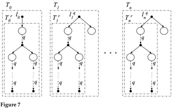
Figure 7
Uqof a generic CF-UGU.
Theorem 4
IfUis incanonical form, thenUqis a forest of exactly|Lq
U|+1 trees, rooted atL q
U∪ {l0}.
RU=defLqU∪ {l0}are called the roots ofU.
Proof.According to the second condition in Definition 12, thenquantifier nodes andl0
are the only nodes with no incoming edge, therefore they form all and the onlyn+1 roots of the graph of a CF-UG. Every other label or hole node must be dominated by one of thosen+1 roots. According to the first condition of Definition 12, the body holes of quantifiers have no outgoing edge, therefore every other node must be either under
the restriction of a quantifier or underh0. 2
Because qeq constraints were introduced by MRS, in Section 7.2, we show that, in practice, all MRS structures generated by MRS’s proposed syntax/semantic interface are in canonical form. Canonical form defines the smallest complete UG over a set of ETs.
Definition 14 (Completeness)
A UG iscompleteif it has a spanning sub-UG in canonical form.
The following set of definitions become handy throughout the rest of this paper.
Definition 15 (Floating Scopal Trees/Restriction Trees/Heart Tree)
We refer to T1,T2,. . .,Tn, the trees in Uq rooted at LqU, as floating scopal trees
(a.k.a. quantifier trees); T1r,Tr2,. . .,Trn, the trees rooted at the restriction hole of the floating scopals, as the restriction trees; and T0, the tree rooted at l0, as the heart
3.1 Equivalence of Qeq and Dominance Relations
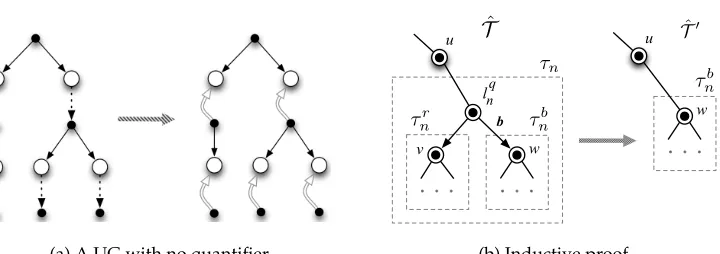
In this section, we show that, for every complete UG, qeq and dominance relations are equivalent. That is, as stated by Theorem 5, if qeq constraints are replaced with dominance relations, the solutions of the UG remain the same. This fact explains why frameworks such as Dominance Graph are able to model scope underspecification even though they only use dominance constraints, and helps to bridge the gap between the two sets of formalisms. We first prove this for the case when there is no quantifier inU.
Lemma 2
Let U be a complete UG with no quantifier. Let ˆU be the UG obtained from U by treating all qeq edges as dominance constraints, that is, DUˆ =DU∪QU and QUˆ =∅.
Every solution ofUis a solution of ˆUand vice versa.
Proof.The first direction is trivial because qeq is a special case of dominance. In order to prove the other direction, consider the leaf label nodes of ˆU (Figure 8(a)). In any solution of ˆU, these label nodes have to be fused to the hole from which they have re-ceived a dominance constraint. Let us fuse these labels, and then, following Theorem 2, collapse the EPs with the fused hole(s) into a single node. We can now apply the same argument to the newly leaf nodes and repeat this until we reach the top (remember that UGs are finite). This shows that every holehof ˆUhas to be fused with the labell where (h,l)∈QU. Becausehis fused directly withl, following the definition of qeq, the
constraint betweenhandlis satisfied, even if it is treated as qeq. This means that ˆT is
also a solution ofU. 2
Theorem 5
LetUbe a complete UG, and ˆUbe the UG obtained fromUby treating all qeq edges as dominance constraints, that is,DUˆ =DU∪QU andQUˆ =∅. Every solution of ˆUis a
solution ofUand vice versa.
(a) A UG with no quantifier
lnq u
v w
ˆ
T
uw
b
⌧n
⌧r
n ⌧nb
⌧nb
ˆ
T0
[image:16.486.56.416.500.627.2](b) Inductive proof
Figure 8
Proof. Because qeq always implies dominance, it is trivial that every solution ofUis a solution of ˆU. Using the lemma and induction onn, the number of quantifiers, we prove the other direction, that is, if ˆT is a solution of ˆU, then it is also a solution ofU.
Letn=0. Because there is no quantifier in ˆT, according to Lemma 2, every holehis fused withlwhere (h,l)∈QU, therefore, every qeq constraint is satisfied.
Now letn>0 andUbe an arbitrary UG withnquantifiers (see Figure 7), and ˆT be a solution of ˆU. Consider the quantifier nodelqwith the longest distance from the root
of ˆT (breaking ties arbitrarily), meaning thatlqdoes not outscope any other quantifier node in ˆT. Without loss of generality, assume thatlq=lqnand use ˆτn, ˆτrn, and ˆτbnto refer
to the trees rooted atlqnand the left and the right child oflqnin ˆT, respectively, as shown
in Figure 8(b). According to Lemma 2:
(i) All qeq constraints in the quantifier tree Trnare satisfied inTˆ.
Now let us remove the quantifier tree rooted atlqnfromUand ˆUand call the resulting
UGsU0and ˆU0, respectively. Accordingly, detach the tree ˆτnfrom ˆT, replace it with ˆτbn and call the new tree ˆT0, as demonstrated in Figure 8(b). ˆT0is a solution of ˆU0, and hence (based on the induction assumption) is a solution ofU0. Therefore, all qeq constraints in U0are satisfied in ˆT0, which also proves:
(ii) All qeq constraints in U0are satisfied inTˆ.
This is because if two nodes are connected with ab-path in ˆT0, they are also connected with ab-path (possibly including an additionalb-edge (lqn,w)) in ˆT.
From (i) and (ii) every (h,l)∈QUis satisfied in ˆT, hence ˆT is a solution ofU. 2
The next section introduces the heart of our framework, the concept of semantic coherence.
4. Coherence
In this section, we introduce the notion of sentence-level semantic coherence based on a simple principle: that every variable introduced in the domain of discourse must contribute to the overall meaning of the sentence. We formally characterize this quality as a property of a UG, and refer to sentences whose interpretation is a coherent UG as coherent sentences. We posit as a general principle of language the requirement that sentences should be coherent. This general principle goes back at least as far as Frege (1923), and is widely accepted, although, because it is not a mathematical statement, it cannot be proved. Our definition of coherent UG, on the other hand, is mathematically precise, and can be used to prove that all coherent sentences are tractable, as we will see in Section 5.
4.1 Mathematical Characterization of Semantic Coherence
ways, either by directly participating in the main predication13 or by participating in
the definition of another relevant variable. If variablexparticipates in the definition of y, we say thatyis (semantically) dependent onx. To summarize, a variablexis relevant if either the heart or another relevant variable depends on it. For example, in the sentence Every child of a politician runs, the variablex, quantified byEvery, is relevant, because it is an argument of the main predication, and the variabley, quantified byA, is relevant, becausexdepends on it. Following these intuitions and given that dependencies in a UG are encoded in the binding (i.e., dominance) constraints, we formally define relevance as follows.
Definition 16 (Dependence/Relevance)
Consider a completeU,14with the top holel0andlqi,l q
j ∈L
q U:
r
lqj (l0, forj=0)dependsonlqi, if (l q
i,u)∈DUfor someuin a restriction
treeTr j.
r
lqi is said to berelevantif
(i) l0depends onlqi; or
(ii) lqj depends onlqi, andlqj is relevant.
Definition 17 (Coherence)
A complete UGUis calledcoherentif everylqi inUis relevant.
Trivially, relevance is closed under the increment of constraint edges, resulting in the following lemma.
Lemma 3
Coherence is closed under the increment of (dominance) constraint edges.
In Manshadi, Allen, and Swift (2009), we defined the notion of semantic de-pendency graph and a property of such graphs called heart-connectedness. Heart-connectedness is nothing but a notational variant of coherence. In this article, we shall use the notion of semantic dependency graph to compare our framework with Hole Semantics (Section 7.3). Therefore, in the rest of this section, we formally define this notion and prove that the two formulations of coherence are in fact equivalent.
Definition 18 (Semantic Dependency Graph)
Given a CF-UG U, we define semantic dependency graph orSDG ofU as SDGU=
(V,E), where
r
V={0, 1,. . .,n}, wheren=|LqU|.r
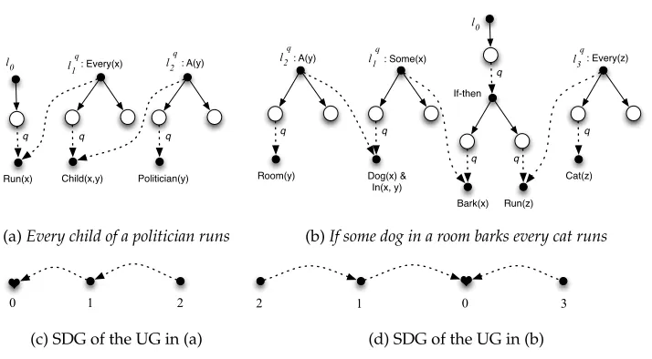
(i,j)∈Eif and only ifi6=j,i>0, and (lqi,u)∈DU, whereuis a node inTjr.Politician(y) : A(y)
Child(x,y) : Every(x)
Run(x)
l 1q l 2q
q l 0
q q
(a)Every child of a politician runs
Dog(x) & In(x, y)
: Some(x)
Room(y) : A(y)
Cat(z) : Every(z)
Bark(x) If-then
Run(z)
q q q
q q
q l 2q l 1q
l 0
l 3q
(b)If some dog in a room barks every cat runs
2 1
0
(c) SDG of the UG in (a)
0 3
1 2
[image:19.486.55.412.63.260.2](d) SDG of the UG in (b)
Figure 9
Constructing semantic dependency graph.
Intuitively, SDGU is obtained by taking the CF-UGUand collapsing its heart and
quantifier trees—that is, each of the treesT0,. . .,Tn—into a single node, resulting in
a directed graphGofn+1 nodes. Figure 9 demonstrates this transformation for two real-life CF-UGs. The dependencies inUare simply encoded in the edges ofG. In other words, ifiis the node ofGcorresponding toTi, an edge fromitojinGmeans thatlqj
(l0, ifj=0) depends onlqi inU. From Definition 18, SDGs aresimplegraphs, that is, (i)
they have no self-loops, and (ii) for everyi,jthere is at most one (directed) edge from itoj. Node 0, which corresponds to the heart of the CF-UG, hence called theheartof SDG, has no outgoing edge, therefore the heart is always a sink node.
Definition 19 (Heart-Connectedness)
A SDGGis calledheart-connectedif every node inGreaches the heart by a directed path. A CF-UGUis calledheart-connected, if SDGUis heart-connected.
Theorem 6
A CF-UGUis coherent if and only if it is heart-connected.
The theorem directly follows from the following lemma.
Lemma 4
The nodelqi is relevant in a CF-UGU, if and only ifireaches the heart in SDGU.
Proof.Following Definition 16, the setRof all the relevant nodes inUcan be constructed as follows:
(a)
2 3
0 1
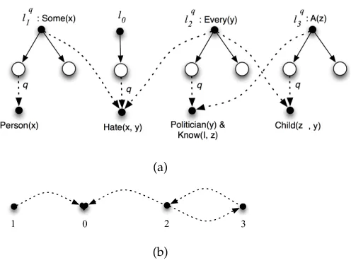
[image:20.486.51.299.60.246.2](b)
Figure 10
UG and SDG forSomebody hates every politician whom I know a child of.
r
R=Snm=0Rm, whereRm(m>0) is the set of nodes thatR(m−1)
depends on.15
Using induction onm, it is easy to see that for every nodelqi ∈R, nodeireaches the heart
in SDGUusing a directed path of lengthm. 2
All examples of UG given so far are acyclic. This may suggest that the SDG of every sentence is acyclic, but this is not the case. As a counterexample, consider the UG in Figure 10, motivated by an example from Hobbs and Shieber (1987). This example shows that coherent UGs form a very broad class of UGs, subsuming other previously proposed classes, as we will see in Section 7. Notwithstanding their broad applicability, coherent UGs can be tractably processed, as we will see in the next section.
5. Tractability
An algorithmic problem arising within the context of constraint-based underspecifica-tion frameworks is to determine whether a given UG has a soluunderspecifica-tion or not. This is called thesatisfiabilityproblem, or, in short,SAT. This becomes important when new con-straints are incrementally added at the deeper levels of language processing. Another closely related problem commonly studied within the same context is to enumerate all possible solutions, the enumerationproblem, or, in short,ENUM. All the constraint-based underspecification frameworks that we have built UG upon (HS, MRS, and DG) are intractable in their general form, meaning that their satisfiability problem is NP-complete. Over the last decade, there has been a series of work on finding a subset of these frameworks that can be solved efficiently. The previously found tractable subset
15 We require thatRm⊂LqU− S(m−1)
is inadequate in that it does not cover all natural language sentences (see Definition 29 in Section 7.1 for details), leaving open the question whether there is a tractable subset with sufficient expressivity. In this section, we answer this question by introducing the largest tractable subset found so far and prove that every coherent sentence, under our linguistically justified notion of semantic coherence, belongs to this subset.
5.1 Dominance Graph
In the previous sections, we showed that for coherent (in fact, complete) UGs, qeq and dominance constraints are equivalent. A UG with only dominance constraints is called a dominance graph, or, in short,DG, which is the core concept of the Dominance Graphs framework. Most of the work on finding a tractable subset of URs has previously been done within the realm of this framework. Because coherent UGs are a subset of dominance graphs, our work is built on top of this work, hence, in this section we only work within this framework.
Remember from Definition 2 that a UG is an 8-tuple hL,H,E,Q,D,T,Lq,Pi. With no qeq constraints, a dominance graph has noQcomponent. As a result, there is no need to distinguish floating scopal (i.e., quantifier) ETs; and hence, there is also no Lq component, which in turn means that there is no designated top ET in dominance graphs. Therefore, all labels can potentially form the root of a solution. We now give a formal definition of dominance graph.
Definition 20 (Dominance Graph)
ADominance Graph, or DG, is a 5-tupleG=hLU,HU,EU,DU,PUiwhere all the
compo-nents are as defined in Definition 2. Because there is no designated top node, analogous to ˜LU, we define ˜LlG=LU− {l}for every label nodel. All the variations of UG defined
in Section 2.2 are defined correspondingly for DG.
It should be noted that in order to build a fusion, we have to first pick an arbitrary labell, and then constructf as a function from ˜LlGtoH. The nodelwill be a root ofTU,f
(the only root, iff is total). Following this definition, every UG can be converted into a DG by dropping the top ET and treating all qeq constraints as dominance constraints.
Definition 21 (DG Counterpart)
Given a UG U, GU, the DG counterpart of U, is obtained by removing the
top ET from U and converting all qeq edges into dominance. More precisely, GU =
hHG,LG,EG,DG,PGiwhereHG=HU− {h0},LG=LU− {l0},EG=EU− {(l0,h0)},DG=
DU∪QU− {(u,v)| {u,v} ∩ {l0,h0} 6=∅},PG=PU.
The following lemma directly results from Theorem 5.
Lemma 5
There is a one-to-one relationship between the solutions of a complete UGUand those of its DG counterpartGU.
Mumble
When
Yawn Not
Speak Or
Mumble
When
Yawn Not
Speak
U Or
U1 U2
Mumble
When
Yawn Not
Speak Or
T1 T2
(a)
(b)
Mumble
When
Yawn Not
Speak Or
T1 T2
(d) (c)
[image:22.486.54.373.66.311.2]T
Figure 11
Recursive construction of solutions.
and we treat it as the mathematical characterization of coherence within the context of DGs. The definition of hypernet is motivated by the definition of (weak) nets (Niehren and Thater 2003), a previously found tractable subset of DG, and it translates our semantically motivated concept of coherence into (a slightly more powerful version of) the already popular structures of DG. Built on top of the fairly complex notion of nets together with the incorporation of heart-connectedness (as the mathematical characteri-zation of coherence), there should be no surprise that the definition of hypernet is quite complex. For this reason, instead of presenting the complete definition at once, we step by step justify our way through the full definition of hypernet.
Remember that our ultimate goal is to efficiently solve (a subset of) DGs. Here is a recursive approach. Pick an ET for the root of the solution and remove it from the DG. Recursively solve each of the remaining smaller DGs and plug the root of the resulting trees into the holes of that ET. Figure 11 demonstrates this procedure and Table 1 lists the steps. In order for this approach to work, each of the resulting subgraphs should be a valid DG. Let us make this intuition formal.
Definition 22 (Sub-DG)
Table 1
Recursive procedure followed in Figure 11.
1: procedureSOLVE(DGG)
2: IfGcontains a single (label) node, return that node as a single-node treeT. 3: Pick an ETE satisfying all the conditions to be the root of a solution, otherwise,
fail.
4: LetGr,Gbbe the twoDGs resulting from the removal ofE(Figure 11(b)).
5: LetTr=SOLVE(Gr),Tb=SOLVE(Gb)
6: BuildT by pluggingTrintohrandTbintohb. 7: returnT.
Politician(y) Child(x,y)
Every(x)
Run(x)
A(y)
(a) DGG
Every(x)
A(y)
Politician(y)
Run(x)
Child(x, y)
T
0(b) SolutionT ofG
Politician(y) Child(x,y)
A(y)
[image:23.486.62.432.230.354.2](c) Sub-DG induced byT0
Figure 12
DG counterpart of the UG forEvery child of a politician runsand a sub-DG of it.
ends are present inG0. Given a solutionT ofGand a subtree16 T0ofT, a sub-DGG0
inducedbyT0is the sub-DG induced by the set of ETs ofT0.
Figure 12 gives an example of these concepts. The following property, which di-rectly follows from the definition, will help in proving the completeness of the recursive method (Section 5.3).
Lemma 6
Consider a DGG, a solutionT ofG, and a subtreeT0 ofT. IfG0 is the sub-DG ofG induced byT0, thenT0is a solution ofG0.
The notion of sub-DG helps in solving DGs recursively, as shown in Figure 12. Depending on whether, at step 3, among all nodes satisfying the conditions, we pick a nodearbitrarilyoriterativelydetermines whether the algorithm will be a SAT algorithm (generating an arbitrary solution on success) or an iterative ENUM algorithm (every branch of which builds one solution). Note that, whereas the total size of the output for ENUM may be exponential, we are interested in bounding its running per solution produced.
In the rest of this section, we form this intuition into a detailed algorithm and define hypernet as a subset of DG for which the algorithm is both sound and complete. Because label-to-hole constraints add another level of complexity, we first ignore those edges and only consider weakly normal DGs. We then adopt the algorithm by Koller and Thater (2007) to take care of label-to-hole constraints.
5.2 Hypernets
A look at the steps in Table 1 reveals that the heart of this procedure is to find the roots of the solutions. The rest is simply recursing on the smaller DGs.
Definition 23 (Freeness)
A labellis said to befreeif it is the root of some solutionT ofG. An ETEis called free if its root is free.
Subsequently, we use some graph theory terminology that we need to define. Remember that two nodes of a digraph areweakly connectedif there is an undirected path between the two. Because weak connectedness is an equivalence relation, it par-titions the graph into equivalence classes each of which is called a weakly connected componentorWCC.
Theorem 7 states some necessary conditions for freeness, but first, we state a lemma that is the key to the proof of this theorem.
Lemma 7
Given a weakly normal DGGand a solutionT ofG, if nodesuandvinGare weakly connected using an undirected pathp, there exists a nodewonpsuch thatwdominates bothuandvinT.
This lemma is analogous to Lemma 3 in Bodirsky et al. (2004). A detailed proof of the lemma can be found there. We are now prepared to prove the theorem.
Theorem 7
LetGbe a weakly normalDGandE be an ET withmholes rooted at labell.lcan be a free label,onlyif
T7a. lhas no incoming (constraint) edge; and
T7b. Every distinct hole ofEis in a distinct WCC inG−l; and
T7c. G−Econsists of at leastmWCCs.
Proof. Let T be a solution rooted at l, h a hole of E, and Gh the WCC of G−l
containingh.
T7a. This condition is trivial.
T7b. Following Lemma 7, every node inGhmust be in the scope ofh(because
inT, but the only possiblewisw=h). BecauseT is a tree, this proves that every two holes ofEbelong to two distinct WCCs.
T7c. This follows from T7b and the fact that no hole may be left unfused. 2
We now look for a subset of DG, for which the conditions in T7a through T7c are not only necessary, but also sufficient. In defining this subset, the following notion from Althaus et al. (2003) plays an important role.
Definition 24 (Hyper-Normal Connectedness)
Given a DGG, ahyper-normal pathis an undirected path with no two consecutive constraint edges emanating from the same node. Nodeuishyper-normally connected to nodevif there is at least one hyper-normal path between the two.Gis called hyper-normally connectedif every pair of nodes inGare hyper-normally connected.
For example, in Figure 13,p2 is a hyper-normal path, butp1 is not. In spite of that,
the whole graph is hyper-normally connected, because even thoughp1is not a
hyper-normal path, there is another hyper-hyper-normal path connecting the same two nodes. The following notion from Thater (2007) will also come in handy.
Definition 25 (Openness)
A label or hole nodeuis called anopen nodeif it has nooutgoingconstraint edge.
For example,lin Figure 14(a) is an open label node andh2in Figure 14(b) is an open
hole.
Definition 26 (Hypernet)
A DGGis called ahypernetif it has a weakly normal spanning sub-DGG0in which for every elementary treeErooted atl:
D26a. Ehas at most one open node.
D26b. Ifl1andl2are two dominance children of a holehofE, thenl1andl2are
hyper-normally connected inG0−h.
D26c. IfEhas no open hole inG0:
[image:25.486.54.226.554.646.2]p1 p2
Figure 13
l
h
1h
2U
1U
2l
h
1h
2U
1U
2(a) (b)
l
h
1h
2U
1U
2 [image:26.486.59.392.63.191.2](c)
Figure 14
Three types of elementary trees: (a) open-root (b) open-hole (c) closed.
r
Each dominance child oflis hyper-normally connected to a hole of EinG0−l.Otherwise (i.e., whenEhas an open hole):
r
All dominance children ofl, not connected to a hole ofEinG0−l,are hyper-normally connected together.
Here, by dominance children ofu, we mean nodesv where (u,v) is a dominance edge. Notice that by enforcing conditions (D26a) through (D26c) on a spanning sub-DG of Grather than Gitself, we allow the hypernet to be closed under the increment of constraint edges. This is in line with the definition of coherence, which imposes only a minimum connectivity, hence, closed under the increment of dominance constraint edges.17 Following condition (D26a), a weakly normal hypernet may have three types of scopal ET, characterized in the following definition.
Definition 27
Given a DGGand an ETE,Eis called
D27a. Open-root: iff only the root ofEis open inG.
D27b. Open-hole: iff only a hole ofEis open inG.
D27c. Closed: iffEhas no open node inG.
Figures 14(a–c) show the three types ofE, respectively. Definition 26 guarantees the following property.
Theorem 8
LetGbe a weakly normal hypernet andEbe an ET ofGwithmholes and rooted atl. If lsatisfies the conditions in Theorem 7,G−Econsists of exactlymWCCs, each of which is a (weakly normal) hypernet.
Proof. Following conditions (D26b) and (D26c),G−Econsists of at mostmWCCs (since the children of each node ofE are hyper-normally connected, they stay connected in G−E). Based on condition (T7c),G−Ehas at leastmWCCs. Therefore,G−Ehas exactly mWCCs. To prove that each of these WCCs is a hypernet, we show that, for any two nodesuandvnot belonging toE, ifuandvare hyper-normally connected inG, they are also hyper-normally connected inG−E. We do so by proving that there is no hyper-normal path betweenuandvinGthat visits some node ofE.
Suppose thatEis an open-hole ET rooted atl(Figure 14(b); a similar line of reason-ing can be used for open-root and closed ETs). Assume to the contrary that there is a hyper-normal pathpbetweenuandvthat visits some node ofE. Because an ET consists of a single label nodelwith some number of holes as children, one of the following three cases holds:
i. pvisits exactly one node ofE.
ii. pvisits (at least) two holes ofE.
iii. pvisitsland exactly one hole ofE.
All three cases result in a contradiction: Case (i) means that p is not hyper-normal; case (ii) shows that E violates condition (T7b); and case (iii) proves that G is not a
hypernet, becauseEviolates condition (D26c). 2
The following corollary will be helpful in the subsequent subsections when stating the relation between heart-connectedness and hyper-connectedness.
Corollary 2
LetGbe a weakly normal hypernet andT be a solution ofG. For any subtreeT0ofT, the sub-DG ofGinduced byT0is a (weakly normal) hypernet.
We are now ready to prove the main result of this subsection.
Theorem 9
If G is a satisfiable weakly normal hypernet, the necessary conditions of freeness (Theorem 7) are also sufficient.
Proof. LetErooted atlbe an ET satisfying the freeness conditions in Theorem 7. Among all the solutions ofG, we pick a solutionT in which the depthdoflis minimal. Using proof by contradiction, we show thatd=0, hence,l is the root of T. Assume to the contrary that d>0, meaning that there is some node l0 outscoping l (Figure 15(a)). Without loss of generality assume thatE has only exactly two holes (Left and Right). We show that at least one of the trees in Figures 15(b,c) is a solution ofG, which means Ghas a solution in which the depth oflis smaller thand—a contradiction!
Figure 15(d) showsGwith the two WCCs ofG−lcalledGL andGR. Note that all
the nodes inT2 andT3have to be inGLandGR, respectively (in the figure,G2 andG3
show subgraphs ofGinduced byT2andT3). In order to show thatTborTcis a solution,
we assume thatTbis not a solution and prove that Tc is. BecauseTb is not a solution,
there are some unsatisfied constraints inTb. However, there are not many constraints
Figure 15
Proof of Theorem 9.
inT2, or inT3are also satisfied inTb). In fact, an unsatisfied constraint can only be in the
form of (l0,l2) or (h0,l2) withh0being the right hole ofl0(the hole to whichlis fused in T), andl2being a label inT2(it is true that a constraint froml0tolis not satisfied inTb
either, but such a constraint does not exist aslis a free node). Becausel2 is inGL and
there is a constraint betweenl0orh0andl2,l0belongs toGLas well.
Similar toTb, in order forTcnot to be a solution, there must be a constraint (l0,v3)
or (h0,v3) violated, wherev3is a node inT3, and hence, inGR. Butl0andh0are inGL, so
such constraints cannot exist. This means there cannot be any unsatisfied constraint in
Tc. This proves thatTcis a solution in whichlhas a lower depth. 2
5.3 SAT and ENUM Algorithms
Following Theorems 8 and 9, Table 2 gives the algorithms forSATandENUM.
Theorem 10
ENUM and SAT are correct for all weakly normal hypernets.
Table 2
SAT and ENUM algorithms for weakly normal hypernets.
1: procedureSOLVE(Weakly normal hypernetG)
2: IfGcontains a single (label) node, return the single-node treeT =({l},{}).
3: Pick an ETEsatisfying the freeness conditions in Theorem 7, otherwise, fail.
.For SAT, pick arbitrarily.
.For ENUM, pick iteratively.
4: Letlbe the root andmthe number of holes ofE.
5: LetG1,G2,. . .,Gmbe WCCs ofG−E. 6: LetTi=SOLVE(Gi) fori=1,. . .,m.
7: Lethibe the hole ofEconnected toGiinG−l, fori=1,. . .,m.
IfEhas an open holehk, letGkbe the WCC not connected to any hole ofE. 8: BuildT by plugging the root ofTiintohi, fori=1,. . .,m.
Proof. Using Theorem 8 and induction on the depth of recursion, it is easy to see that if ENUM or SAT return a treeT,T is a solution ofG. This proves that ENUM and SAT are sound.
An inductive proof is used to prove the completeness as well. By completeness, we mean that any solution ofGisarbitrarily/iterativelygenerated by SAT/ENUM. Let
T be an arbitrary solution ofG rooted at the ET E, andT1,. . .,Tn be the subtrees of T under the holes h1,. . .,hn of E. Following Lemma 6 (Section 5.1), in order for T
to be a solution of G, the subtrees T1,. . .,Tn must be the solutions to G1,. . .,Gn, the
WCCs ofG−E connected to h1,. . .,hn inG−l, respectively (ifE has an open holehk,
Gk will be the WCC not connected to any hole of E inG−l). Based on the induction
assumption,T1,. . .,Tnare arbitrarily/iteratively generated by SOLVE(). Therefore,T is
also arbitrarily/iteratively generated. 2
The running time of the algorithms is proportional to the number of recursive calls to SOLVE(), that is,O(|L|). At each call, it takesO(|G|) to find the set of free ETs (Bodirsky et al. 2004) and also to computeG−Efor some free ETE, where|G|=def |L|+|H|+|E|+ |D|. Therefore, SAT (as well as each branch of ENUM) runs inO(|L||G|) time, meaning that the worst-case time-complexity of SAT (and each branch of ENUM) is quadratic in the size ofG.
This result is for weakly normal hypernets—that is, when there are no label-to-hole constraints. Kallmeyer and Romero (2008) demonstrate cases where having such constraints is meaningful. The function of label-to-hole constraints is quite counter-intuitive. Consider the two ETsEandE0rooted atlandl0and containing holeshandh0,
respectively. A label-to-hole constraint (l0,h) results in two types of solutions: those in whichl0dominatesl, and those in whichl0is plugged intoh. The algorithm presented in Table 2 may be easily modified to solve any hypernet by taking care of label-to-hole constraints after a free ETE is picked. At step 3.1, every label-to-hole constraint (l,h0) may be replaced with (l,l0). Every (l0,h) is taken care of by pluggingl0intoh. This latter step results in a stacked ET, but we know how to convert this into a standard ET without affecting the set of solutions (Theorem 2). Note that, here, we have to recursively take care of the incoming constraints to the holes ofE0. Koller and Thater (2007) prove that adding such a step to the algorithm increases the complexity from quadratic to cubic, when label-to-hole constraints exist. Following this discussion, we have:
Lemma 8
Every hypernet can be solved in polynomial time.
Table 3
Viterbi algorithm for weakly normal hypernets. We use a functionsigto determine the dynamic programming signature of a solution, an arrayδto maintain the best scores found for partial solutions, and an arraybestto maintain the best partial solutions themselves. Arraysδandbest are indexed by a subgraphGand a signature. We usebest[G] to denote the set of all the best solutions found forG, regardless of their signature.
1: procedureVITERBI(Weakly normal hypernetG)
2: δ[G]← −∞ .Initialize for all signatures
3: best[G]← ∅
4: if Gcontains a single (label) nodethen
5: T =({l},{})
6: δ[G,sig(T)]←score(T)
7: best[G,sig(T)]←T
8: return
9: foreach ETEsatisfying the freeness conditions in Theorem 7do
10: Letlbe the root andmthe number of holes ofE.
11: LetG1,G2,. . .,Gmbe WCCs ofG−E. 12: Fori=1,. . .,m
13: if not definedbest(Gi)then
14: VITERBI(Gi)
15: for (T1,. . .,Tm)∈best[G1]× · · · ×best[Gm]do
16: Lethibe the hole ofEconnected toGiinG−l, fori=1,. . .,m.
17: IfE has an open holehk, letGkbe the WCC not connected to any hole of E.
18: BuildT by plugging the root ofTiintohi, fori=1,. . .,m. 19: if score(T)> δ[G,sig(T)]then
20: δ[G,sig(T)]←score(T)
21: best[G,sig(T)]←T
The first approach is simply to use the ENUM algorithm as the framework for search in statistical scope disambiguation systems. We can use ENUM to list solutions meeting the hard constraints and score each solution individually. This rescoring ap-proach may take exponential time in the worst case, but may be an effective algorithm when the hard constraints leave a tractable number of solutions in practice. This ap-proach has the advantage that it can take advantage of arbitrary weighted constraints, also known as features, in scoring candidate solutions.
As an example of applying the ENUM together with dynamic programming, sup-pose that the weighted features of the statistical system are restricted to consider only an ET and the hole into which it is plugged. In this case, we can construct a dynamic programming chart indexed by the subset of ETs covered by a partial solution, and the identity of the ET at the root of the partial solution. The size of this chart isO(n2n) in the number of ETs—still exponential in the worst case. However, as with the more general features, the ENUM algorithm, memoizing recursive calls with the chart, can take ad-vantage of the hard constraints of the UG to lower the time complexity in practice. More generally, we can define a dynamic programming chart indexed by whatever features of the partial solution are distinct to the statistical model, and memoize recursive calls to ENUM according to this dynamic programming structure.
More efficient algorithms for finding the highest scoring solution may be possible, and are an important area for future work. Our polynomial-time SAT algorithm does not translate directly into a Viterbi algorithm that is polynomial in the size of the input UG. However, we emphasize that for any NP-hard problem with hard constraints, the weighted generalization is also NP-hard. Therefore, identifying a subset of UGs that is tractable with hard constraints makes it possible to attempt to find efficient algorithms for weighted constraints.
5.4 Coherence and Tractability
In this section, we show that coherent UGs are a subset of hypernets. Remember that the key notion for defining hypernets is hyper-normal connectedness and for coher-ence is connectedness. Therefore, as the first step, we demonstrate how heart-connectedness relates to hyper-normal heart-connectedness.
Theorem 11
LetUbe a CF-UG. Ifiis connected tojthrough a directed path inSDGU, thenlqi andl q j
are hyper-normally connected inGU.
Proof. First assume thatiis directly connected tojthrough the edge (i,j). This means that there is a dominance constraint (lqi,u) inUfor some nodeuofTjr. Being the root of Tj,lqj reachesuby a directed, and hence hyper-normal, pathp. The pathpi,jbetweenlqi
andlqj, which is the concatenation ofpand (lqi,u), is therefore hyper-normal.
Now assume that i is connected to j through a directed path −→d. Following the previous result,lqi is connected tolqj inGUthrough a pathp, which is the concatenation
of hyper-normal paths corresponding to the edges of −→d . Because, at each point of concatenation, one of the two edges is a solid edge (Figure 16(a)), the concatenation
remains hyper-normal. 2
This theorem proves that heart-connectedness subsumes hyper-normal connected-ness for the following reason. Given any two arbitrary nodesu and v belonging to treesTiandTj, bothiandjcan reach the heart through some directed path inSDGU.
Therefore,lqi and lqj are hyper-normally connected to the heart through hyper-normal pathsp1andp2, as shown in Figure 16(b). Concatenatingp1andp2while taking out the
Ti Tj Tk T0
l0' liq lj
q
lk q
(a) Hyper-normal paths betweenlqi,lqj, andlqk
u
v
heart w
p p
1
p 2
[image:32.486.56.421.63.216.2](b) Constructingpfromp1andp2 Figure 16
The relation between heart-connectedness and hyper-normal connectedness.
Corollary 3
IfUis a heart-connected CF-UG,GU is hyper-normally connected.
We now have the tools to prove our main theorem.
Theorem 12
For every coherent UGU,GUis a hypernet, and hence, tractable.
Proof.Uis coherent, hence according to Theorem 6,Uhas a heart-connected canonical form sub-UGU0. In the following proof, we show thatU0is a hypernet. Because hyper-nets are closed under the increment of constraint edges, it follows thatUis a hypernet. LetEbe an arbitrary ET inGU0rooted atl.
T12a. (Proof of condition D26a) We need to show thatEhas at most one open hole.
Eis of one of the following three types:
r
Floating scopal. BecauseU0is complete, the only possibly openhole ofEis its body hole. SinceU0is coherent, the root ofEqmust
also be closed.
r
Fixed scopal. BecauseU0is complete,Ehas no open hole, hence,the only potentially open node is the root ofE.
r
Non-scopal.Ehas a single label node, hence, its only potentiallyopen node.
T12b. (Proof of condition D26b) We need to prove the following statement. Ifl1andl2are two dominance children of a holehofE,l1andl2are
quantifiers have no outgoing constraint and every other hole has exactly one).
T12c. (Proof of condition D26c) First consider the case whereEhas no open hole. BecauseU0is a CF-UG,Emust be either a fixed scopal or a non-scopal ET. In either case,lhas no dominance children inG0U, hence, the statement is vacuously true. Now consider the case w