Fast 3D Reconstruction using Structured Light Methods

(1)

Fast 3D Reconstruction using Structured Light Methods

RODRIGUES, Marcos <http://orcid.org/0000-0002-6083-1303>

Available from Sheffield Hallam University Research Archive (SHURA) at: http://shura.shu.ac.uk/5037/

This document is the author deposited version. You are advised to consult the publisher's version if you wish to cite from it.

Published version

RODRIGUES, Marcos (2011). Fast 3D Reconstruction using Structured Light Methods. In: International Conference on Medical Image Computing and Computer Assisted Intervention, Toronto, Canada, 18-22 September. (Unpublished)

Copyright and re-use policy

See http://shura.shu.ac.uk/information.html

Sheffield Hallam University Research Archive

(2)

Tutorial on 3D Surface Reconstruction in Laparoscopic Surgery

Marcos A Rodrigues

Geometric Modelling and Pattern Recognition Research Group Sheﬃeld Hallam University, Sheﬃeld, UK

www.shu.ac.uk/gmpr

(3)

Marcos A Rodrigues – Fast 3D Reconstruction using Structured Light Methods

Tutorial on 3D Surface Reconstruction in Laparoscopic Surgery. 22nd September ,Toronto, Canada

Structured light scanning

Chapter 2 – Prior work

and featureless is debatable. It may contain a number of strong features such as the eyes and eyebrows, but may also have smooth featureless parts such as the cheeks and forehead. However since the saliency of features on arbitrary (unknown) faces can vary significantly, and since stereo matching is a complex and challenging task, we decide not to focus on this scanning method.

2.1.4 Structured light scanning

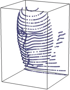
The method ofstructured light scanning[35] operates by projecting a pattern of light onto the target surface. A camera then records the pattern as it reflects from the surface. The shape of the captured pattern is combined with the spatial relationship between the light source and the camera, to determine the 3D position of the surface along the pattern. Figure 2.2 shows an example where the pattern consists of a single horizontal line. A synthetic recorded image of a grid pattern of dots is also shown.

camera

light source

target object image captured_{by camera} _{pattern of dots}projecting a

(a) (b)

Figure 2.2: A structured light scanner projects a pattern of light, in this case a horizontal stripe, onto the target surface. A camera records the reflected pattern. The image marked (b) shows a captured pattern of dots.

Early structured light systems originated from laser range finding and used a single stripe of laser light to measure a particular “slice” of the target object [99], as shown in Figure 2.2. The target surface would then be moved in relation to the scanner to measure another part, thus generating a sequence of surface parts that could be stitched together. The availability

16

1.  Operates by projecting a pattern of light onto the target surface

2.  A camera records the pattern as it reﬂects from the surface

3.  The shape of the captured pattern is combined with the spatial relationship

(4)

Important characteristics

•  The cost of the system is fairly low as it requires only a light

source, such as a slide or LCD projector, and a standard digital camera (for a visible spectrum solution).

•  The speed of acquisition allows for rapid, almost instantaneous,

acquisition.

•  The accuracy of the system can be controlled by the projected

pattern and camera resolution.

•  The process can be made completely non-‐intrusive by

implementing a near-‐infrared (NIR) emitter and an NIR sensitive sensor to capture the image.

•  As with stereo vision, the system is constrained only by the

(5)

Coding schemes

a)  Time-‐multiplexing projects a series of luminance patterns over

time so that every recorded point is encoded by a sequence of intensities. Only for motionless objects.

b)  Colour coding stripes are used to diﬀerentiate between the

recorded stripes. It can cause problems where the surface exhibits weak or ambiguous reﬂection properties.

c)  Uneven distribution in stripe width reduces the resolution and

can cause diﬃculties on a surface with variable depth. d)  Projecting uncoded stripes is the preferred method.

Chapter 2 – Prior work

suited. It is opaque, fairly diﬀuse [34] and, apart from small features, fairly smooth and monotone. Specular highlights (or glossiness) may occur due to the presence of oily sebum on the skin [87], but we have not found this to be a major concern.

Various projected patterns have been considered such as dots [97], horizontal and vertical stripes [32, 54, 101], and diagonal stripes [14]. An advantage of stripes over dots, and the reason why we choose stripes, is that an improved sample resolution is achievable. Note that for the camera to sense pattern deformity the stripes need to be normal (not parallel) to the plane spanned by the camera and projector axes (this follows from the epipolar constraint which we discuss in section 3.5.3).

For a direct and unambiguous mapping between image space and 3D space it is important to know which captured pattern element corresponds to which projected element. Many coding schemes have been proposed to distinguish between different captured stripes (see [107] for a review). Figure 2.3 shows some examples. One proposed scheme, called time-multiplexing, projects a series of luminance patterns over time so that every recorded point is encoded by a sequence of intensities [32, 122]. This method can be robust and accurate but, because it requires multiple scans over time, is suitable only for motionless objects. To avoid the need for multiple scans single static patterns have been proposed where colour [102], stripe width [13, 81], or a combination of both [134] is used to differentiate between the recorded stripes. An uneven distribution in stripe width, however, reduces the resolution and can cause difficulties on a surface with variable depth. Colour coding can cause problems as well where the surface exhibits weak or ambiguous reflection properties.

(a) time-multiplexing (b) colour coding (c) variable width (d) uncoded stripes

Figure 2.3: Diﬀerent coding schemes (a)–(c) which may aid in solving the correspondence problem in a structured light scanning system.

(6)

Advantages of uncoded stripes

•  It allows for “one-‐shot” scanning, such that the acquisition is

nearly instantaneous and can be performed at frame rate (unlike time-‐multiplexing methods),

•  the maximum resolution from a single scan can be achieved

with a suﬃciently dense pattern of stripes (unlike variable width coding), and

•  it can be applied consistently to a variety of diﬀerent object

(7)

A scanner layout

Chapter 3 – Structured light scanning

3.1 THE LAYOUT OF OUR SCANNER

Figure 3.1 illustrates the basic concept of a structured light scanner which utilizes a pattern of horizontal stripes. A projector is utilized to cast the pattern onto the surface of a target object, and a camera captures an image of the scene. Information retrieved from the image is combined with the geometric relationship between the projector and camera in order to reconstruct a cloud of points in 3D. This is possible because each stripe corresponds to a sheet of light originating from the centre of the projector lens and the image reveals where those sheets hit the target surface.

recorded image

←−

projector camera

target object

[image:7.842.502.624.129.286.2]

reconstructed point cloud

Figure 3.1: A series of parallel stripes is projected onto the surface of an object. A recorded image of this scene reveals the shape of the surface along those stripes, and can be used to reconstruct a 3D point cloud.

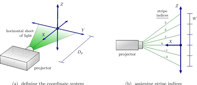
We define a Cartesian coordinate system spanning a 3D space in which the scanner is cali-brated and in which the surface can be reconstructed. Refer to Figure 3.2(a). The axes are chosen in relation to the projector such that: the X-axis coincides with the central projector

axis; the X–Y plane coincides with the horizontal sheet of light cast by the projector; and

the system origin is at an arbitrary, but fixed and known, distance Dp >0 from the centre of the projector lens. We call the space spanned by these axes thesystem space.

29

A series of parallel stripes is projected onto the surface of an

object. A recorded image of this scene reveals the shape of

the surface along those stripes, and can be used to

(8)

Deﬁning the coordinate system

a)  We deﬁne a coordinate system in relation to the projector.

b)  Indices are assigned to planes emanating from the projector.

The planes project to evenly spaced stripes on the Y –Z plane. Chapter 3 – Structured light scanning

projector X

Y Z

Dp

horizontal sheet of light

projector

X Z

W

−2

−1 0

1 2 3

stripe indices

[image:8.842.212.631.106.288.2]

(a) defining the coordinate system (b) assigning stripe indices

Figure 3.2: (a) We define a coordinate system in relation to the projector. (b) Indices are assigned to planes emanating from the projector. The planes project to evenly spaced stripes on theY–Z plane.

Each projected stripe lies in a specific plane that originates from the projector, and the position and shape of a certain stripe in such a plane depend on the surface it hits. Figure 3.2(b) shows the arrangement of these planes as viewed down theY-axis. They are all parallel to theY-axis and their intersections with theY–Z plane are evenly spaced. To discriminate between the planes we assign successive indices as shown. Note that the horizontal plane containing the projection axis (and therefore also theX-axis) has an index of 0. The distance W between two consecutive stripes on the Y–Z plane can be measured and enables us, for example, to write the point of intersection between the Z-axis and a plane with index n as (0,0, W n) in system coordinates.

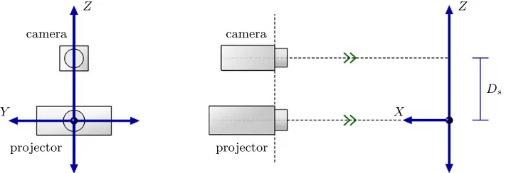
The position of the camera is fixed in system space on top of the projector, as shown in Figure 3.3. We require that:

• the central camera axis lies in the X–Z plane, and is parallel to the X-axis (therefore

also to the projector axis);

• the centre of the camera lens is at point (Dp,0, Ds) in system space, with Ds>0; • and the camera is not “tilted” (rotated about its central axis) with respect to the

projector, such that any point in theX–Z plane is captured to the central image column.

(9)

The relationship between camera and projector

The camera is positioned at a distance Ds above the projector so that its central axis lies in the X–Z plane and is parallel to the

projector axis.

camera

projector

Y

Z

camera

projector

X

Z

[image:9.842.247.606.155.277.2]

Ds

Figure 3.3: The camera is positioned at a distanceDs above the projector so

that its central axis lies in the X–Z plane and is parallel to the projector axis.

Note that we fix the camera to be parallel to the projector. This diﬀers from conventional structured light systems, such as those described in [35, 47, 54, 91, 101, 122, 134], where the camera and projector axes angle towards each other and intersect at a certain point close to the target surface. A number of reasons why we favour the parallel configuration is presented at the end of this chapter (section 3.5).

3.2 MAPPING IMAGE POINTS TO SURFACE POINTS

Next we derive formulae for mapping points on stripes in the recorded image to their cor-responding surface points. These formulae will be used to map points on all the captured stripes in the image, thereby producing a point cloud in system space that represents a dis-crete sampling of the target surface. A mesh structure can then be fitted to such a point cloud to produce a surface model. The process of mapping points in the image to points in system space consists of the following three steps:

(1) an image point (or pixel) is transformed to a point on the sensor plane of the camera in system space;

(2) the eﬀects of radial lens distortion are corrected for;

(3) the intersection of the appropriate camera ray and the plane cast from the projector, corresponding to a specific stripe index, is found.

(10)

Mapping image points to surface points

Three steps:

1.  An image point (or pixel) is transformed to a point on the

sensor plane of the camera in system space;

2.  the eﬀects of radial lens distortion are corrected for;

3.  the intersection of the appropriate camera ray and the plane

(11)

Image space to system space

The position of a pixel in the image at row r and column c is

transformed to coordinates (v,h), and then to a point p in system space.

Note that we express the pixel size speciﬁcally as PF so that F cancels in some of the equations that follow.

3.2.1 Image space to system space

The recorded image is generated in thesensor plane of the camera which is behind the lens perpendicular to the camera axis. It may, for example, consists of an array of charge-coupled device (CCD) sensors that capture light and convert it into electrical signals which are then used to produce a digital image. We consider such an image as a matrix withM rows andN

[image:11.842.195.623.107.258.2]

columns containing as elements the greyscale information (integer values between 0 and 255) of pixels. We will write (r, c) to denote the pixel at row r and columnc.

Figure 3.4 illustrates how a pixel (r, c) in the image is mapped to a point p on the sensor

plane of the camera in system space. The pixel is first transformed to centred coordinates (v, h), with

v=r₋1₂(M + 1) and h=c₋1₂(N + 1). (3.1)

Since the focal point of the camera is located at (Dp,0, Ds) in system space, the centre of the

sensor plane is located at c = (Dp+F,0, Ds). Here F is the focal length of the camera, as

illustrated in Figure 3.4(c). Assuming that each pixel on the sensor plane is a square of size

P F _×P F, we can write the coordinates of pointp as

p=c+ (0,₋hP F, vP F). (3.2)

Note that we express the pixel size specifically as P F so that F cancels in some of the

equations that follow.

M

N

r

c

(a) image space

1 2M 1 2N v h (b) centred F camera ←−p

(c) system space

Figure 3.4: The position of a pixel in the image at row r and column c is

transformed to coordinates (v, h), and then to a point p in system space.

32

3.2.1 Image space to system space

The recorded image is generated in the sensor plane of the camera which is behind the lens

perpendicular to the camera axis. It may, for example, consists of an array of charge-coupled device (CCD) sensors that capture light and convert it into electrical signals which are then

used to produce a digital image. We consider such an image as a matrix with M rows and N

columns containing as elements the greyscale information (integer values between 0 and 255)

of pixels. We will write (r, c) to denote the pixel at row r and column c.

Figure 3.4 illustrates how a pixel (r, c) in the image is mapped to a point p on the sensor

plane of the camera in system space. The pixel is first transformed to centred coordinates (v, h), with

v = r ₋ 1₂(M + 1) and h = c ₋ 1₂(N + 1). (3.1)

Since the focal point of the camera is located at (Dp,0, Ds) in system space, the centre of the

sensor plane is located at c = (Dp + F,0, Ds). Here F is the focal length of the camera, as

illustrated in Figure 3.4(c). Assuming that each pixel on the sensor plane is a square of size

P F _× P F, we can write the coordinates of point p as

p = c + (0,₋hP F, vP F). (3.2)

Note that we express the pixel size specifically as P F so that F cancels in some of the

equations that follow.

M

N

r

c

(a) image space

1 2M 1 2N v h (b) centred F camera

←−

p

(c) system space

Figure 3.4: The position of a pixel in the image at row r and column c is

transformed to coordinates (v, h), and then to a point p in system space.

(12)

Radial distortion correction

A recorded image can suﬀer from radial lens distortion, which can be corrected (in an estimated sense) by a transformation.

We use the Tsai camera model:

k is the lens distortion coeﬃcient which should be determined for a speciﬁc camera and lens prior to scanning.

3.2.2 Radial distortion correction

The coordinates of a surface point will be found by triangulation. To accomplish this we need to model the camera as an idealpinhole camera and assume the lens of the camera projects light rays linearly onto its sensor. In practice however a lens typically distorts the image slightly [46]. This distortion is radial meaning that it is greater for points further away from the centre of the image. Figure 3.5 illustrates the eﬀect on a synthetic image.

⇒

V

H

(vu, hu) (vd, hd)

r

Figure 3.5: A recorded image can suﬀer from radial lens distortion, which can be corrected (in an estimated sense) by a transformation.

We will use the Tsai camera model [119] to correct for radial lens distortion. The model approximates the undistorted position (vu, hu) of a pixel from its distorted location (vd, hd)

given by (3.1), as follows:

hu =hd(1 +kr2),

vu =vd(1 +kr2),

with r=

�

h2_d+v2_d. (3.3)

In the model k is the lens distortion coeﬃcient which should be determined for a specific

camera and lens prior to scanning. A value of k = 0 would imply no distortion, and the

greaterk is the greater the distortion.

We assume that the lens of the projector does not distort its output. This is true for many LCD projectors which automatically apply correction by an inverse distortion. It can also be verified by observing that the projection of a rectangle onto a plane normal to the projector axis remains a rectangle (i.e. the edges remain straight and rectilinear).

33

3.2.2 Radial distortion correction

The coordinates of a surface point will be found by triangulation. To accomplish this we need

to model the camera as an ideal pinhole camera and assume the lens of the camera projects

light rays linearly onto its sensor. In practice however a lens typically distorts the image

slightly [46]. This distortion is radial meaning that it is greater for points further away from

the centre of the image. Figure 3.5 illustrates the eﬀect on a synthetic image.

⇒

V

H

(vu, hu) (vd, hd)

r

Figure 3.5: A recorded image can suﬀer from radial lens distortion, which can be corrected (in an estimated sense) by a transformation.

We will use the Tsai camera model [119] to correct for radial lens distortion. The model

approximates the undistorted position (vu, hu) of a pixel from its distorted location (vd, hd)

given by (3.1), as follows:

hu = hd(1 +kr2),

vu = vd(1 +kr2),

with r =

�

h2_d +v_d2. (3.3)

In the model k is the lens distortion coeﬃcient which should be determined for a specific

camera and lens prior to scanning. A value of k = 0 would imply no distortion, and the

greater k is the greater the distortion.

We assume that the lens of the projector does not distort its output. This is true for many LCD projectors which automatically apply correction by an inverse distortion. It can also be verified by observing that the projection of a rectangle onto a plane normal to the projector axis remains a rectangle (i.e. the edges remain straight and rectilinear).

(13)

Mapping from (v, h, n) to (x, y, z)

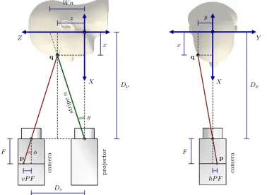
The geometry of the scanner, as viewed down the Y -‐axis (left) and down the Z-‐axis (right), is used to map points in the image to

corresponding surface points in system space Chapter 3 – Structured light scanning

3.2.3 Mapping from (v, h, n) to (x, y, z)

After a point in the captured image is corrected for in terms of radial distortion and mapped to a point in system space, it is mapped to a surface point. Figure 3.6 shows schematic diagrams of the scanner and target object in system space as viewed downY-axis (left) and Z-axis (right). The system parametersW,Dp,Ds and F are also shown.

A pixel (r, c) on a captured stripe is transformed to pointpon the sensor plane. It then follows

that the corresponding surface point q = (x, y, z) lies on the line through p and the focal

point of the camera. Suppose, for now, it is also known that the particular captured stripe has indexn(we consider the significant problem of establishing stripe indices in Chapter 4).

Then q is also on the plane parallel to the Y-axis through points (Dp,0,0) and (0,0, W n). The surface pointqis therefore the intersection of that plane and the camera ray.

X Z

Dp

W n

Ds

vP F F

x z

stri p e

n

p

q

camera _pro

jector

θ

φ

X

Y

Dp

hP F F

x

y

p q

[image:13.842.220.598.99.375.2]

camera

Figure 3.6: The geometry of the scanner, as viewed down the Y-axis (left)

and down theZ-axis (right), is used to map points in the image to

correspond-ing surface points in system space.

(14)

Mapping surface points

By triangulation:

Note that by construction

Combining these expressions:

Based on those arguments we can find expressions for the coordinates x, y and z of point q.

Similar triangles in Figure 3.6 (left) yield

z

Dp −x

= W n

Dp

=_⇒ z = W n

Dp

(Dp −x), (3.4)

and

vP F

F =

Ds −z

Dp − x

=_⇒ z = Ds − vP (Dp −x). (3.5)

Note that by construction Dp > x, Dp > 0 and F > 0.

Combining (3.4) and (3.5) yields

W n

Dp

(Dp −x) = Ds −vP (Dp − x) =⇒ x = Dp −

DpDs

vP Dp+ W n

, (3.6)

which can be substituted into (3.4) to give

z = W n

Dp

�

Dp− Dp +

DpDs

vP Dp +W n

�

= W nDs

vP Dp +W n

. (3.7)

Also, by similar triangles in Figure 3.6 (right),

y

Dp −x

= hP F

F =⇒ y = hP(Dp −x) =

hP DpDs

vP Dp +W n

. (3.8)

We can show that vP Dp + W n �= 0 by referring to Figure 3.6 (left), and observing that

vP = tan(φ) and ₋W n/Dp = tan(−θ). Since both φ and θ are in (−π/2,π/2) it follows

that vP = ₋W n/Dp if and only if φ = −θ. But if φ = −θ then the ray emanating from the

camera is parallel to the plane containing stripe n, so that they can never intersect at a point

q. Therefore such a scenario will never occur, and vP Dp +W n �= 0. In fact, for the camera

ray to intersect the stripe plane at a point in front of the scanner (i.e. such that x < Dp), the

angle φ must be strictly larger than ₋θ, so that

vP Dp+ W n > 0. (3.9)

To recapitulate,

x = Dp(1−K),

y = hP DpK,

z = W nK,

with K = Ds

vP Dp + W n

. (3.10)

These formulae can be applied to map a pixel with distortion corrected image coordinates (v, h) that lies on stripe n, to its corresponding surface point (x, y, z) in system space.

35 Chapter 3 – Structured light scanning

Based on those arguments we can find expressions for the coordinates x, y and z of point q. Similar triangles in Figure 3.6 (left) yield

z Dp −x

= W n Dp

=_⇒ z = W n Dp

(D_p ₋x), (3.4)

and

vP F F =

D_s ₋z

D_p ₋x =⇒ z =Ds−vP (Dp −x). (3.5) Note that by construction Dp > x, Dp >0 and F > 0.

Combining (3.4) and (3.5) yields W n

Dp (

D_p ₋x) = D_s ₋vP (D_p ₋x) =_⇒ x =D_p ₋ DpDs vP Dp +W n

, (3.6)

z = W n D_p

�

Dp −Dp +

D_pD_s vP D_p +W n

�

= W nDs

vP D_p +W n. (3.7)

Also, by similar triangles in Figure 3.6 (right), y

D_p ₋x = hP F

F =⇒ y =hP(Dp −x) =

hP D_pD_s

vP D_p +W n. (3.8)

We can show that vP D_p + W n _�= 0 by referring to Figure 3.6 (left), and observing that vP = tan(φ) and ₋W n/D_p = tan(₋θ). Since both φ and θ are in (₋π/2,π/2) it follows that vP =₋W n/D_p if and only if φ = ₋θ. But if φ = ₋θ then the ray emanating from the

q. Therefore such a scenario will never occur, and vP D_p +W n _�= 0. In fact, for the camera ray to intersect the stripe plane at a point in front of the scanner (i.e. such that x < Dp), the

vP Dp +W n > 0. (3.9)

To recapitulate,

x =D_p(1₋K), y =hP D_pK, z =W nK,

with K = Ds vP Dp +W n

. (3.10)

Based on those arguments we can find expressions for the coordinates x, y and z of point q. Similar triangles in Figure 3.6 (left) yield

z

Dp−x

= W n

Dp

=_⇒ z = W n

Dp

(Dp−x), (3.4)

and

vP F

F =

Ds −z

Dp −x

=_⇒ z = Ds −vP (Dp−x). (3.5)

Note that by construction Dp > x, Dp > 0 and F > 0.

Combining (3.4) and (3.5) yields

W n

Dp

(Dp− x) = Ds −vP (Dp−x) =⇒ x = Dp −

DpDs

vP Dp +W n

, (3.6)

z = W n

Dp

�

Dp −Dp +

DpDs

vP Dp +W n

�

= W nDs

vP Dp +W n

. (3.7)

Also, by similar triangles in Figure 3.6 (right),

y

Dp −x

= hP F

F =⇒ y = hP(Dp−x) =

hP DpDs

vP Dp +W n

. (3.8)

We can show that vP Dp + W n �= 0 by referring to Figure 3.6 (left), and observing that vP = tan(φ) and ₋W n/Dp = tan(−θ). Since both φ and θ are in (−π/2,π/2) it follows

that vP = ₋W n/Dp if and only if φ = −θ. But if φ = −θ then the ray emanating from the

q. Therefore such a scenario will never occur, and vP Dp +W n �= 0. In fact, for the camera

ray to intersect the stripe plane at a point in front of the scanner (i.e. such that x < Dp), the

vP Dp +W n > 0. (3.9)

To recapitulate,

x = Dp(1−K),

y = hP DpK,

z = W nK,

with K = Ds

vP Dp +W n

. (3.10)

(15)

Fixing system variables

1.  Choose a calibration plane:

1.  This plane will coincide with the Y –Z plane in system space and the

scanner will be positioned and calibrated in relation to it. 2.  Calibrate the projector [Dp, W, centre stripe]:

1.  The projector is positioned in front of the calibration plane such that its

central axis is normal to that plane. The parameter Dp can then be

measured directly as the perpendicular distance between the focal point of the projector and the calibration plane.

2.  The parameter W is measured as the spacing between two consecutive

stripes on the calibration plane. Greater accuracy can be achieved by measuring a width W∗ over m stripes, and calculating W = W∗/m.

3.  It is also necessary to identify and mark one reference stripe of a known

index, so that the other stripes in the image can be assigned indices

(16)

Fixing system variables

3.  Calibrate the camera [P]: a horizontal distance d is marked on

the calibration plane and recorded by the camera. The number of pixels, p, between the endpoints of d is determined. Then by triangulation:

[image:16.842.220.616.113.255.2]

X Y Dp F pP F d camera

Figure 3.7: The central vertical column of the projection pattern should be captured to the central image column (left), regardless of depth. Similar trian-gles can be used (right) to determine the value of parameter P.

and in the exact centre of the image both vertically and horizontally. An image of this chart is recorded, and two points (v1, h1) and (v2, h2) on the same vertical grid line are selected

such that h1 �=h2. Since they lie on the same vertical grid line they should have the same

undistorted h-value, hence by (3.3),

h1

�

1 +k(h2₁+v₁2)�=h2

�

1 +k(h2₂+v2₂)� =_⇒ k= h2−h1

h3₁−h3₂+h1v2₁−h2v₂2

. (3.11)

The procedure can be repeated for diﬀerent pairs of points in the image, and along horizontal grid lines, which can then also give an indication of the consistency and suitability of the distortion model.

The last parameter to determine isP which indicates the size of a pixel on the sensing plane of

the camera. Refer to Figure 3.7 (right). A horizontal distance dis marked on the calibration

plane and recorded by the camera. The endpoints of this distance are corrected by (3.3), and the number of pixels, p, between them is determined. Then by similar triangles,

pP F F =

d Dp

=⇒ P = d pDp

. (3.12)

This concludes the calibration procedure.

X Y Dp F pP F _d camera

Figure 3.7: The central vertical column of the projection pattern should be

captured to the central image column (left), regardless of depth. Similar trian-gles can be used (right) to determine the value of parameter P.

and in the exact centre of the image both vertically and horizontally. An image of this chart is recorded, and two points (v1, h1) and (v2, h2) on the same vertical grid line are selected

such that h1 �= h2. Since they lie on the same vertical grid line they should have the same

undistorted h-value, hence by (3.3),

h1 �1 + k(h2₁ + v₁2)� = h2 �1 + k(h2₂ + v₂2)� =⇒ k = h2 − h1

h3₁ ₋ h3₂ + h1v₁2 − h2v₂2

. (3.11)

The procedure can be repeated for diﬀerent pairs of points in the image, and along horizontal grid lines, which can then also give an indication of the consistency and suitability of the distortion model.

The last parameter to determine is P which indicates the size of a pixel on the sensing plane of

the camera. Refer to Figure 3.7 (right). A horizontal distance d is marked on the calibration

plane and recorded by the camera. The endpoints of this distance are corrected by (3.3), and the number of pixels, p, between them is determined. Then by similar triangles,

pP F

F =

d

Dp

=_⇒ P = d

pDp.

(3.12)

This concludes the calibration procedure.

(17)

Choosing system parameter values

Dp: the distance between the projector and the system origin

W: the width between successive stripes on the calibration plane

Ds: the distance between the camera and the projector

P: the pixel size on the sensor plane of the camera

(18)

Viewing volume

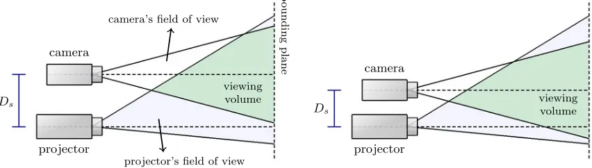
The viewing volume of the scanner is the space visible by both the camera and the projector. This volume is likely to increase as Ds is decreased.

Thus, Ds should be ﬁxed as small as possible, i.e. have the camera as close to the projector as possible, because it may (1) increase the viewing volume and (2) decrease the likelihood of occlusions.

The remaining parameter that can be modified is Ds. We propose to fix Ds as small as

possible, i.e. have the camera as close to the projector as possible, because it may (1) increase the viewing volume and (2) decrease the likelihood of occlusions. These two concepts are discussed in more detail next.

The target surface has to be in the field of view of both the projector (so that stripes can be projected onto it) and the camera (so that the projected stripes can be recorded). The space visible from both the projector and the camera is called the viewing volume of the scanner. Usually the viewing volume can be bounded by a plane parallel to the Y–Z plane, because of a maximum focus distance of either the projector or the camera. Figure 3.8 illustrates. It seems, from the figure, that as Ds is decreased the viewing volume increases. There may

however be a lower bound on an optimal Ds due to the asymmetric field of view of the

projector. It depends on the specific equipment used, but as a general rule of thumb we say that a smallDs should yield a large viewing volume.

b

oun

ding

pla

ne

Ds

projector camera

viewing volume

−→

camera’s field of view

←−

projector’s field of view

Ds

projector camera

[image:18.842.199.625.102.223.2]

viewing volume

Figure 3.8: The viewing volume of the scanner is the space visible by both the camera and the projector. This volume is likely to increase asDs is decreased.

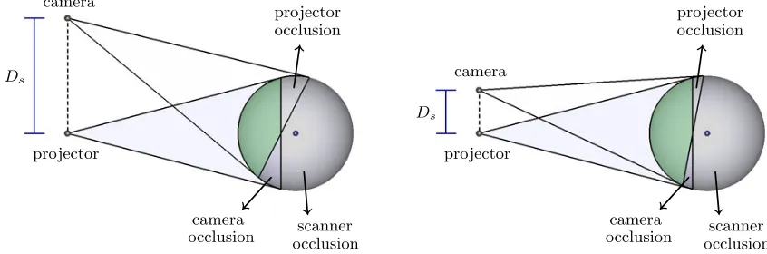
The second reason for choosing a small distance between the camera and projector is to reduce the likelihood ofocclusions, which are regions of the target surface not visible from either the projector or the camera, or both. We define the following three types:

• camera occlusion : a region visible from the projector but not from the camera; • projector occlusion : a region visible from the camera but not from the projector; • scanner occlusion : a region not visible from either the projector or the camera.

(19)

Occlusions

•  camera occlusion : a region visible from the projector but not

from the camera;

•  projector occlusion : a region visible from the camera but not

from the projector;

•  scanner occlusion: a region not visible from either the

projector or the camera.

The remainder of the surface, that which is visible from both the camera and projector, is the

scannable region. Occlusions are a well-known problem in surface scanning (see e.g. [31, 91]).

[image:19.842.183.606.108.248.2]

Such regions cannot be reconstructed because suﬃcient information cannot be retrieved.

Figure 3.9 shows an example of a spherical target surface, and the diﬀerent occlusion types.

As the camera is moved closer to the projector the occluded regions reduce in size, and

(in theory) setting Ds to zero would yield a maximum scannable area, and no camera or

projector occlusions. It seems therefore thatDsshould be fixed as small as possible to reduce

the likelihood of occlusions and increase the scannable area.

projector camera

Ds

←−

scanner occlusion

−→

projector occlusion

←−

camera occlusion

projector camera

Ds

←−

scanner occlusion

−→

projector occlusion

←−

camera occlusion

Figure 3.9: Occlusions, i.e. areas not visible from the projector and/or the camera, can be reduced by positioning the camera closer to the projector.

Of course, the size and location of occlusions depend on the shape of the specific target

surface. The eﬀect of an increasing Ds on the scannable region of a synthetic face model is

shown in Figure 3.10†_{, for an arrangement similar to the one in Figure 3.1. It illustrates that,}

as expected, the area of the scannable region decreases as Ds is increased.

†_{The pictures in Figure 3.10 were generated by testing angles. Suppose the focal points of the projector and}

camera are positioned atpandcrespectively. A surface pointxwith outward normalnis then visible from

the projector if the line segment between pand x does not intersect the surface, and if the angle between

(p₋x) and nlies in (₋90◦_,₉₀◦_{), i.e. if} _n_·_(p₋_x) _>_{0. Similarly,} _x _{is visible from the camera if the line}

segment between c andx does not intersect the surface and n_·(c₋x) >0. The scannable region is then

the union of all points visible from both the projector and the camera. We did not take into account their

bounded fields of view which would reduce the scannable area even more.

(20)

Occlusions and angle of projection

•  Scannable area is decreased as Ds is increased

•  Size of scannable region may also depend on angle of projection

Ds= 50 Ds= 100 Ds= 250 Ds= 400 Ds= 600 Ds= 1,000

Figure 3.10: The area of the scannable region decreases as the distance Ds (shown in mm) between the camera and projector is increased, as illustrated here on a synthetic face model.

3.3.3 The angle of projection

So far we have considered as the projection pattern an array of evenly spaced horizontal stripes. As mentioned in section 2.1.4, an advantage of continuous stripes over a dot pattern is the improved sample resolution attained. We now consider the angle at which these stripes are projected on the face.

For the camera to record a sensible deformation caused by the shape of the target surface, and for the mapping in (3.10) to be applicable, the stripes have to be projected parallel to theY-axis. Figure 3.7 (left) illustrates this well, where the projected horizontal stripe reveals

[image:20.842.165.629.285.461.2]

the shape of the surface it hits while no deformation is visible for the vertical one. We can however freely rotate the entire scanner, i.e. the projector and camera as a combined whole, which enables the projection of stripes vertically, diagonally, or indeed at any desired angle. An optimal angle of projection depends entirely on the shape of the target surface.

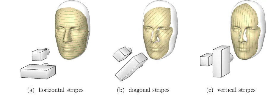
Figure 3.11 illustrates the eﬀect of rotating the scanner on the size of the scannable region of a face. Because of the sides of the face and nose, both large surface regions which are almost parallel to theX–Z plane, the horizontal configuration shown in Figure 3.11(a) seems

favourable. The projection of vertical stripes requires the camera to be next to (as opposed to on top of) the projector with respect to the face, which can easily cause the sides of the face and nose to be occluded from either the projector or the camera.

42

(a) horizontal stripes (b) diagonal stripes (c) vertical stripes

Figure 3.11: An illustration of the diﬀerence in size of the scannable region (shown in dark) of a typical face attained from projecting (a) horizonal, (b) diagonal and (c) vertical stripes.

3.4 ANALYSIS OF THE RESOLUTION

In this section we explore the resolution of the scanner. By resolution we mean the smallest measurable distance that the scanner is able to recognize, or into how small an interval the reconstructed points can be resolved. It is therefore related to the sample density, and also gives an indication of the achievable degree of accuracy.

The stripes project to a discrete set of curves on the surface of the target object, and the captured image consists of a discrete array of pixels in which we locate recorded stripes. The resolution of the scanner would therefore be directly related to the spacing of the projected stripes and the resolution of the pixel space. For a theoretical surface point we will measure the change (e.g. inmm) caused by a perturbation of a single sample unit, which can be either a stripe index or one pixel. We distinguish between the following three resolutions:

(1) thevertical resolution measured along theZ-axis, aﬀected by the stripe index;

(2) thehorizontal resolution measured along the Y-axis, aﬀected by the horizontal

dimen-sion of the pixel space;

(3) thedepth resolution measured along the X-axis, aﬀected by the vertical dimension of

the pixel space.

(21)

Resolution

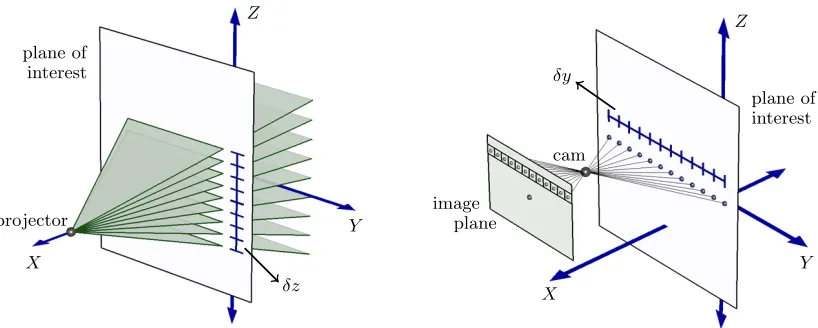
•  The vertical resolution (left) of the scanner is aﬀected by the

spacing of the projected stripes. The horizontal resolution (right) is dependent on the horizontal dimension of the pixel space.

Refer to Figure 3.12 (left). The vertical resolution is dependent on the spacing of the stripes and clearly also on the depth, or location in the X-direction, of the target surface. Consider

an arbitrary surface point (x, y, z) on stripen, and letδzdenote the change of this point along

the Z-axis caused by perturbing the stripe index from n to n+ 1. It follows from similar

triangles that

δz= W Dp

(Dp−x). (3.15) This value is the smallest measurable distance (i.e. resolution) of the scanner along theZ-axis,

and it gets smaller as the target surface is moved closed to the projector.

X Y Z projector plane of interest ← −

δz _X

Y Z cam plane of interest ←− δy image plane

Figure 3.12: The vertical resolution (left) of the scanner is aﬀected by the spacing of the projected stripes. The horizontal resolution (right) is dependent on the horizontal dimension of the pixel space.

For the horizontal resolution refer to Figure 3.12 (right). One row of pixels maps to a uni-formly spaced row of points in a particular fixed depth. Consider one such point (x, y, z)

coinciding with pixel (v, h) in the image, and let δy denote the change of the surface point

along the Y-direction caused by moving fromh toh+ 1. Similar triangles yield

δy=P(Dp−x). (3.16) This expresses the smallest measurable horizontal distance (resolution) of the scanner along the Y-axis. Again, this distance decreases as the target surface is moved nearer to the

projector.

Refer to Figure 3.12 (left). Thevertical resolution is dependent on the spacing of the stripes and clearly also on the depth, or location in theX-direction, of the target surface. Consider

an arbitrary surface point (x, y, z) on stripe n, and letδz denote the change of this point along

the Z-axis caused by perturbing the stripe index from n to n + 1. It follows from similar

triangles that

δz = W Dp

(Dp−x). (3.15)

This value is the smallest measurable distance (i.e. resolution) of the scanner along theZ-axis,

δz _X

along the Y-direction caused by moving from h to h+ 1. Similar triangles yield

δy =P(Dp−x). (3.16)

This expresses the smallest measurable horizontal distance (resolution) of the scanner along the Y-axis. Again, this distance decreases as the target surface is moved nearer to the

projector.

44

Refer to Figure 3.12 (left). The vertical resolution is dependent on the spacing of the stripes and clearly also on the depth, or location in the X-direction, of the target surface. Consider

an arbitrary surface point (x, y, z) on stripe n, and letδz denote the change of this point along

the Z-axis caused by perturbing the stripe index from n to n+ 1. It follows from similar

triangles that

δz = W Dp

(Dp −x). (3.15)

This value is the smallest measurable distance (i.e. resolution) of the scanner along theZ-axis,

δz _X

along the Y-direction caused by moving from h to h+ 1. Similar triangles yield

δy =P(Dp−x). (3.16)

This expresses the smallest measurable horizontal distance (resolution) of the scanner along the Y-axis. Again, this distance decreases as the target surface is moved nearer to the

projector.

44

The ratio between the horizontal and vertical resolutions is given by

δz δy =

W

P Dp

, (3.17)

which, with our current system parameters of Dp = 790mm, P = 0.0006 and W = 3.08mm,

yields a value of about 6.5. Therefore a local region of the reconstructed surface, where the depth is approximately constant, would be roughly 6.5 times more densely sampled in the horizontal dimension (along a stripe) than in the vertical (across the stripes).

Next we investigate the depth resolution, measured along the X-axis, which depends on the

vertical dimension of the pixel space. If a captured stripe has no vertical variation in the pixel space it implies that the target surface along that stripe has no variation in depth. As the depth of a particular surface point on a stripe changes the corresponding pixel of that stripe moves in the vertical direction (i.e. up or down).

Consider a surface point (x, y, z) on stripe n coinciding with pixel (v, h) in the image. We

aim to find an expression that measures the diﬀerence in depth, δx, of this point caused by

perturbing v to v+ 1, as Figure 3.13 (left) illustrates. Using the formula for x in (3.10),

δx = DpDs

vP Dp+W n −

DpDs

(v+ 1)P Dp+W n

= P Dp2Ds

[vP Dp+W n][(v+ 1)P Dp +W n]

. (3.18)

projector camera

image plane

stripe n

[image:21.842.214.623.104.268.2]

1 p ixe l δx X Z x x� A B C D E F G H image plane 1p x 1p x n1 n2

Figure 3.13: The depth resolution is measured as the change δx along the

X-axis caused by a perturbation of one pixel in the vertical direction. It can

be shown that for a given X-position, δx is independent of the stripe index.

(22)

Building 3D models

•  The image contains a darker stripe which is the centre of the system

•  Steps to 3D reconstruction: locate stripes, index stripes, map to 3D

space.

Chapter 4 – Building 3D face models

[image:22.842.131.728.94.282.2]

including sub-pixel estimation, the incorporation of black stripes, generating a mesh surface from the output 3D point cloud and mapping stripe-free texture onto it.

Figure 4.1 shows an image of a face recorded by our structured light scanner. The dense pattern of horizontal stripes can be seen in the close-up (left). The single darker stripe across the upper lip is a reference stripe which has a known index. The algorithms we discuss in this chapter are designed to establish arelative indexing, and in section 4.6.1 we will use the reference stripe to shift from relative to absolute indices.

Figure 4.1: A captured image in which the projected stripes can be seen. A close-up of an area around the nose tip and right nostril is shown on the left.

In Chapter 3 we derived equations for mapping a single pixel in such an image to its corre-sponding point in system space. The process of reconstructing an entire surface consists of the following three steps, illustrated in Figure 4.2 on a small image region:

(1) pixels in the image that contain the vertical centres of stripes are located;

(2) these pixels are indexed, by which we mean a stripe indexnis allocated to each (in the

figure the diﬀerent indices are depicted as diﬀerent colours);

(3) every stripe pixel now has a position (v, h) and an index n, and the mapping (3.10) is

applied to each to determine a collection of points in system space that can be connected by a mesh surface.

54 Chapter 4 – Building 3D face models

captured image (1) locate stripe pixels (2) index stripes (3) map to 3D space

Figure 4.2: The stripes in a 2D image captured by the scanner have to be (1)

located and then (2) indexed in order to (3) reconstruct a 3D surface.

4.1 LOCATING STRIPES IN THE IMAGE

[image:22.842.269.560.100.268.2]

Firstly we need to locate the stripes in the image. This can be achieved by a simple and fast column-by-column scan through the image, marking potential stripe pixels along the way. Figure 4.3 illustrates the basic principle on a small image region. Potential stripe pixels are

determined aslocal maxima in the greyscale luminance values of every column. The output

of the procedure can be a binary matrix P such thatP(r, c) is 1 if pixel (r, c) is marked as a

potential stripe pixel, and 0 otherwise.

column

image

grey

scale

row _output

Figure 4.3: Stripe pixels are determined as local maxima in the greyscale

values of every column in the image.

[image:22.842.203.639.335.446.2]

(23)

Locating stripes

•  Stripe pixels are determined as local maxima in the greyscale

values of every column in the image:

captured image (1) locate stripe pixels (2) index stripes (3) map to 3D space

Figure 4.2: The stripes in a 2D image captured by the scanner have to be (1)

located and then (2) indexed in order to (3) reconstruct a 3D surface.

4.1 LOCATING STRIPES IN THE IMAGE

Firstly we need to locate the stripes in the image. This can be achieved by a simple and fast column-by-column scan through the image, marking potential stripe pixels along the way. Figure 4.3 illustrates the basic principle on a small image region. Potential stripe pixels are

determined aslocal maxima in the greyscale luminance values of every column. The output

of the procedure can be a binary matrixP such thatP(r, c) is 1 if pixel (r, c) is marked as a

potential stripe pixel, and 0 otherwise.

column

image

grey

scale

row _output

Figure 4.3: Stripe pixels are determined as local maxima in the greyscale

values of every column in the image.

We define a local maximum primarily to be any pixel (r, c) satisfying

A(r, c) > A(r ₋ 1, c) and A(r, c) > A(r + 1, c). (4.1)

Here A(r, c) indicates the greyscale value of a pixel (r, c). To reduce the eﬀects of noise in the

image we can set a threshold � below which local maxima are ignored. Our algorithm also

has an amplitude threshold α which indicates the smallest permissible diﬀerence between the

luminance values of a local maximum and its preceding local minimum.

The complete pseudo-code of our procedure for locating stripe pixels is given in Appendix B.

It traverses every pixel of every column in an input M _× N image once, without retracing,

[image:23.842.210.648.105.222.2]

and the computational complexity is therefore linear in the number of pixels. In Chapter 6 we provide some experimental results on the performance and speed of our methods in a biometric setting (where large numbers of faces need to be scanned and recognized).

Figure 4.4 shows the located stripe pixels for the image in Figure 4.1. The next step is to index these pixels, i.e. to decide which of the located stripe pixels correspond to which of the projected stripes. Finding correct indices may be rather simple for flat and “uncomplicated” surfaces but, as the close-up in Figure 4.4 suggests, a definitive solution can be much harder to determine in areas where the curving or bending of the target surface causes discontinuities in the recorded stripes.

Figure 4.4: The located stripes for the image in Figure 4.1. A close-up of the same area around the nose is shown on the left.

We define a local maximum primarily to be any pixel (r, c) satisfying

A(r, c)> A(r−1, c) and A(r, c)> A(r+ 1, c). (4.1)

HereA(r, c) indicates the greyscale value of a pixel (r, c). To reduce the eﬀects of noise in the image we can set a threshold � below which local maxima are ignored. Our algorithm also

has an amplitude thresholdα which indicates the smallest permissible diﬀerence between the

luminance values of a local maximum and its preceding local minimum.

The complete pseudo-code of our procedure for locating stripe pixels is given in Appendix B. It traverses every pixel of every column in an input M ×N image once, without retracing, and the computational complexity is therefore linear in the number of pixels. In Chapter 6 we provide some experimental results on the performance and speed of our methods in a biometric setting (where large numbers of faces need to be scanned and recognized).

Figure 4.4 shows the located stripe pixels for the image in Figure 4.1. The next step is to index these pixels, i.e. to decide which of the located stripe pixels correspond to which of the projected stripes. Finding correct indices may be rather simple for flat and “uncomplicated” surfaces but, as the close-up in Figure 4.4 suggests, a definitive solution can be much harder to determine in areas where the curving or bending of the target surface causes discontinuities in the recorded stripes.

Figure 4.4: The located stripes for the image in Figure 4.1. A close-up of the same area around the nose is shown on the left.

(24)

Indexing the stripes

•  Starting from the centre stripe, diﬀerent indices are depicted as

alternating colours in a repeating sequence

•  A number of algorithms have been implemented based on ﬂood

ﬁlling (Robinson), MST-‐Maximum Spanning Tree (Brink)

•  This is a problem that can be improved

Figure 4.11: Result of applying the MST indexing algorithm on the stripe pixel array in Figure 4.4. Diﬀerent indices are depicted as alternating colours in a repeating sequence, and the same area around the nose is shown on a larger scale.

A remaining issue is that of the connectivity of the graph G. A tree that spans all the

vertices in G can be found only if G is connected, such that every possible pair of vertices

is connected by a series of edges. Since no relationship can be established between two disconnected components ofG, there is also no conceivable way (in an uncoded pattern) to

relate their indices. For this reason we will always find an MST of the largest connected component. The image in Figure 4.4, for example, contains a number of remote vertices in the bottom right corner that could not be indexed.

This concludes the description of the MST indexing algorithm for establishing indices in an uncoded structured light scanning system. The method should be far less likely to cause errors than those mentioned in the previous section. The result is aﬀected neither by a specific starting point nor by the order in which individual stripe pixels are visited, and a single missing stripe pixel can no longer have a major impact on the outcome. However, as is shown in the next section, there is a problem inherent to the indexing of uncoded stripe patterns. We claim that in general this problem cannot be solved without incorporating some additional distinguishing information in the projected stripes.

(25)

Undetectable index shifts

•  Sudden drop in

surface depth

•  Critical depth

changes

4.5 UNDETECTABLE INDEX SHIFTS

An image which causes our indexing algorithm to assign incorrect indices to some stripe pixels is shown in Figure 4.12(a). The problem occurs in an area around the nose. A close-up of this region is shown in (b) and the stripe pixels in (c). A number of indices determined by the MST algorithm is shown in (d) and a correct indexing in (e). The reason for the incorrect indexing is quite clear. Parts of two adjacent stripes appear as one continuing stripe in the image, meeting where the arrow points in Figure 4.12(d). The MST indexing algorithm unknowingly joins these pixels together in a singlewe–connected group and proceeds to index

them with the same index. If the edge of the nose were able to create a break in that seemingly continuous stripe, as is illustrated in (e), the algorithm can index correctly.

We call the phenomenon observed in Figure 4.12 which causes incorrect indexing an unde-tectable index shift. In this section we first establish when it can occur, and then argue why it is quite likely to arise in the scanning of faces. We also discuss a number of approaches for dealing with the problem.

−→

←− edge of nose

(a) captured image

(b) close-up (c) stripe pixels

[image:25.842.240.732.98.513.2]

(d) incorrect indexing (e) correct indexing

Figure 4.12: For this image the MST algorithm indexes incorrectly across

the edge of the nose. This is due to a sudden drop in surface depth (from the nose to the cheek) which causes two diﬀerent stripes to align vertically.

67

4.5.1 Critical depth changes

We aim to find conditions under which an undetectable index shift may occur, i.e. when parts of two stripes appear on the same row in the recorded image. Figure 4.13 (left) shows two adjacent stripes n and n+ 1 projected onto a target surface across an abrupt drop in the

depth. Suppose that this change in surface depth, which we denote by ∆x, causes the left

part of stripen+ 1 and the right part of stripento be captured to equal vertical coordinates

in the image, as shown.

cam

projector

∆x

stripen

stripen+1

view from the camera

n

n+1 n

n+1 A B C D E F G H n1

n1+1 n2 n2

+1

Figure 4.13: An abrupt change ∆xin surface depth (left) causes two succes-sive stripes n and n+ 1to align from the camera’s point of view (middle). It can be shown that the value of∆x is independent of n(right).

We call ∆x a critical change in depth and proceed to derive an explicit expression for it.

Consider surface pointA on stripe n+ 1before the drop in surface depth, and surface point B on stripenafter the drop in depth. These points are assumed to map to the same vertical

coordinate, say v, in the image. If we define x to be the depth of A and x� the depth of B

then, using (3.10),

∆x=x₋x�=Dp

�

1− Ds

vP Dp+W(n+ 1)

� −Dp

�

1− Ds vP Dp+W n

�

. (4.8)

From equations (3.4) and (3.5) we have