Obstacle Detection with Ultrasonic Sensors and Signal Analysis Metrics

(1)

Obstacle Detection with Ultrasonic Sensors and Signal

Analysis Metrics

GIBBS, Gerard, JIA, Huamin and MADANI, Irfan

<http://orcid.org/0000-0002-0339-0636>

Available from Sheffield Hallam University Research Archive (SHURA) at:

http://shura.shu.ac.uk/24880/

This document is the author deposited version. You are advised to consult the

publisher's version if you wish to cite from it.

Published version

GIBBS, Gerard, JIA, Huamin and MADANI, Irfan (2018). Obstacle Detection with

Ultrasonic Sensors and Signal Analysis Metrics. Transportation Research Procedia,

28, 173-182.

Copyright and re-use policy

See

http://shura.shu.ac.uk/information.html

(2)

ScienceDirect

Available online at www.sciencedirect.com

Transportation Research Procedia 28 (2017) 173–182

www.elsevier.com/locate/procedia

International Conference on Air Transport – INAIR 2017

2352-1465  2017 The Authors. Published by Elsevier B.V.

Peer-review under responsibility of the scientific committee of the International Conference on Air Transport – INAIR 2017. 10.1016/j.trpro.2017.12.183

10.1016/j.trpro.2017.12.183 2352-1465

Peer-review under responsibility of the scientific committee of the International Conference on Air Transport – INAIR 2017. Available online at www.sciencedirect.com

ScienceDirect

Peer-review under responsibility of the scientific committee of the INAIR 2017.

INAIR 2017

Obstacle Detection with Ultrasonic Sensors and Signal Analysis

Metrics

Gerard Gibbs

a

_*

_,

_{Huamin Jia}

_b,

_{Irfan Madani}

b

a _{Department of Aerospace, Mechanical and Electronic Engineering,Institute of Technology Carlow, Ireland}

bCentre for Aeronautics, SATM, Cranfield University, England

Abstract

One of the basic tasks for autonomous flight with aerial vehicles (drones) is the detection of obstacles within its flight environment. As the technology develops and becomes more robust, drones will become part of the toolkit to aid maintenance repair and operation (MRO) and ground personnel at airports. Currently laser technology is the primary means for obstacle detection as it provides high resolution and long range. The high intensity laser beam can result in temporary blindness for pilots when the beam targets the windscreen of aircraft on the ground or on final approach within the vicinity of the airport. An alternative is ultrasonic sensor technology, but this suffers from poor angular resolution. In this paper we present a solution using time-of-flight (TOF) data from ultrasonic sensors. This system uses a single commercial 40 kHz combined transmitter/ receiver which returns the distance to the nearest obstacle in its field of view, +/- 30 degrees given the speed of sound in air at ambient temperature. Two sonar receivers located either side of the transmitter / receiver are mounted on a horizontal rotating shaft. Rotation of this shaft allows for separate sonar observations at regular intervals which cover the field of view of the transmitter / receiver. To reduce the sampling frequency an envelope detector is used prior to the analogue-digital-conversion for each of the sonar channels. A scalar Kalman filter for each channel reduces the effects of signal noise by providing real time filtering (Drongelen, 2017a). Four signal metrics are used to determine the location of the obstacle in the sensors field of view:

1. Maximum (Peak) frequency

2. Cross correlation of raw data and PSD 3. Power Spectral Density

4. Energy Spectral Density

Results obtained in an actual indoor environment are presented to support the validity of the proposed algorithm.

* Corresponding author. Tel.: +353 59 9175459.

E-mail address: gibbsg@itcarlow.ie.

Available online at www.sciencedirect.com

ScienceDirect

INAIR 2017

Obstacle Detection with Ultrasonic Sensors and Signal Analysis

Metrics

Gerard Gibbs

a

_*

_,

_{Huamin Jia}

_b,

_{Irfan Madani}

b

a _{Department of Aerospace, Mechanical and Electronic Engineering,Institute of Technology Carlow, Ireland}

bCentre for Aeronautics, SATM, Cranfield University, England

Abstract

One of the basic tasks for autonomous flight with aerial vehicles (drones) is the detection of obstacles within its flight environment. As the technology develops and becomes more robust, drones will become part of the toolkit to aid maintenance repair and operation (MRO) and ground personnel at airports. Currently laser technology is the primary means for obstacle detection as it provides high resolution and long range. The high intensity laser beam can result in temporary blindness for pilots when the beam targets the windscreen of aircraft on the ground or on final approach within the vicinity of the airport. An alternative is ultrasonic sensor technology, but this suffers from poor angular resolution. In this paper we present a solution using time-of-flight (TOF) data from ultrasonic sensors. This system uses a single commercial 40 kHz combined transmitter/ receiver which returns the distance to the nearest obstacle in its field of view, +/- 30 degrees given the speed of sound in air at ambient temperature. Two sonar receivers located either side of the transmitter / receiver are mounted on a horizontal rotating shaft. Rotation of this shaft allows for separate sonar observations at regular intervals which cover the field of view of the transmitter / receiver. To reduce the sampling frequency an envelope detector is used prior to the analogue-digital-conversion for each of the sonar channels. A scalar Kalman filter for each channel reduces the effects of signal noise by providing real time filtering (Drongelen, 2017a). Four signal metrics are used to determine the location of the obstacle in the sensors field of view:

1. Maximum (Peak) frequency

2. Cross correlation of raw data and PSD 3. Power Spectral Density

4. Energy Spectral Density

Results obtained in an actual indoor environment are presented to support the validity of the proposed algorithm.

* Corresponding author. Tel.: +353 59 9175459.

(3)

174 Gerard Gibbs et al. / Transportation Research Procedia 28 (2017) 173–182 2 Gerard Gibbs, et. al. / Transportation Research Procedia 00 (2017) 000–000

Keywords: Kalman filter, Lomb Algorithm, Cross correlation, Envelope detector, and Energy power density;

1. Introduction

The term “drone” and the abbreviations “UAV” (Unmanned Air Vehicle) and “RPAS” (Remotely Piloted Air

Systems) have entered our vocabulary over the last decade. The defence industry refers to their aircraft as UAV’s, while the civil and commercial aviation sector uses RPAS. The visual and print media have adopted the term “drone” to cover all types of unmanned aircraft, from children’s toys to aircraft costing millions of euros.

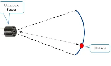
[image:3.544.181.359.302.408.2]

Navigation of these drones in an unknown environment requires the use of many different types of sensors to provide the on board flight controller with data on velocity, position, obstacle distance and orientation. Considerable research has been conducted using LIDAR for range and obstacle detection while on board cameras have been used to implement optical flow as a means of detecting obstacles within the image. Optical sensors are sensitive to light and the use of cameras tends to be computationally expensive, resulting in the use of possible ground stations to aid the on board drone processor. An alternative is the use of ultrasonic sensors which are suitable for close range detection up to ten metres and provides multiple range measurements per second. The advantage of these sensors being that they are inexpensive, have low power consumption and can operate in environmental conditions where other sensors would fail, for example, smoked filled environment. The resolution can be as low as 60 degrees, meaning that they cannot identify the angular location of an obstacle within the sensors field of view as shown in Fig 1.

Fig. 1 Sensor field of view

The main contribution in this paper is to examine the raw data received from a number of sonar receivers and how this can be processed to improve the angular resolution for obstacle detection.

2. Related work

(4)

Gerard Gibbs et al. / Transportation Research Procedia 28 (2017) 173–182 175

Gerard Gibbs, et. al. / Transportation Research Procedia 00 (2017) 000–000 3

under the UAV. To improve the detection angle two sensors are used for one half of the same angle, hence 12 to cover 360 degrees. This can lead to instability due to sonar returns to different receivers within the bank. Using this type of permanent mounting may not provide optimal for obstacle detection since the ideal angle of the sensor to the obstacle surface needs to within 20 degrees, this can lead to problematic surfaces not being detected at all or with the necessary reliability.

An improved detection system proposed by Gageik et al. (2015) uses both ultrasonic and infrared sensors to complement each other for obstacle detection. Using this combination of sensors, it is now possible to detect hard and soft obstacles in the field of view of the UAV. A total of 16 infrared consisting of 8 both for long and short range and 12 ultrasonic sensors providing redundant 360 degree coverage. They divide the obstacle detection into two tasks, sensing and situation awareness. The sensing task receives data from two categories of sensors, main data and reference. The main data being the ultrasonic and infrared, while reference are optical flow and inertial measurement. The reference sensors can support the main sensor selection since the changes in distance should hold a strong correlation to the position changes of the UAV. The novel part of their approach is the use of a weighted filter (WF), which fuses the data from the multiple of sensors in preference to using the Kalman filter which is complex and computationally expensive. One approach proposed by Choset et al. (2003) for a ground robot was the Arc- Transversal Median algorithm (ATM) for obstacle detection. This considers several intersections on an arc as a robot moves within its environment as shown in Fig. 2.

Fig.2 Robot range arc intersections

Where many of the arcs that model the sensor intersect, then the probability of there not being a point of reflection from the obstacle is low. Due to system noise within the environment and sensor these intersection will form a cluster of points which can then provide an approximation of the location of the object along the arc. The weakness of ATM for UAV applications is the need to provide accurate odometry and the ability to stop the vehicle when making a measurement to the obstacle as the distance travelled determines the location of the arc intersection at the transversal

angle (30°). A means of improving the performance of a sensing system is to combine the data from a range of different sensors, this is known as sensor fusion. Caasenbrood (2006) explored the use of ultrasonic sensors combined with IMU measurements to implement UAV pose estimation using a variation of the Kalman filter. No emphasis was placed on obstacle detection or angular resolution within the view of the sensor.

3 System Design

(5)

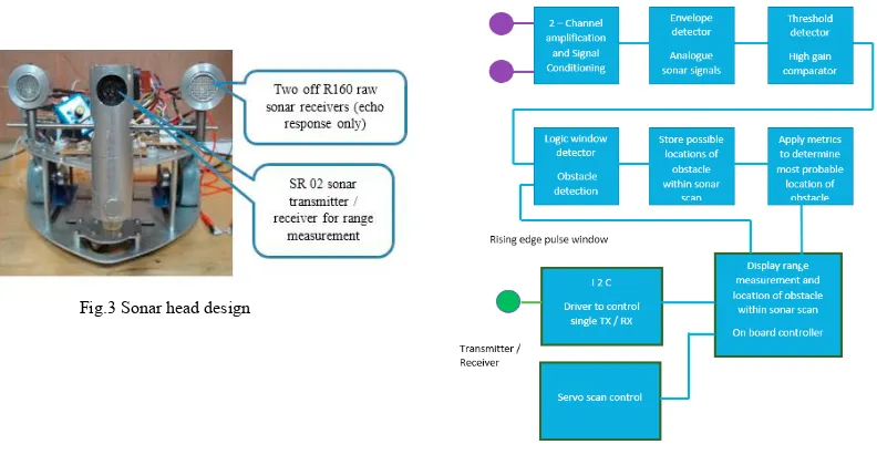
[image:5.544.81.477.80.290.2]

Fig.3 Sonar head design

Fig.4 Sensor head electronics

[image:5.544.162.382.378.497.2]

Fig. 5 shows the output from one of the sonar receivers and the output when this signal is routed through a hardware envelope detector. This simple solution avoids the complexity and processing overhead of using the Hilbert algorithm to implement the envelope detector This allows for a lower sampling rate in the region of 10 kHz compared to in excess of 80 kHz if sampling the raw sonar analogue signal

Fig 5 Raw data and envelope detector

4 Lomb – Scargle Periodgram

The Lomb-Scargle periodgram algorithm is used to perform spectral analysis of a signal with non-uniform intervals. An example of such a signal is the human heartbeat (ECG) which tends to be somewhat irregular (Delane et al., 2016). The algorithm estimates the energy within the signal at a frequency band centred on a frequency, f by fitting a sinusoidal model to the signal. This is accomplished using a means of least squares. The sequence of non-uniform observations (tn, x (n)) is fitted with a model.

(6)

Such that the estimation error is reduced to a minimum:

𝐸𝐸 = ∑[𝑃𝑃𝑛𝑛− 𝑥𝑥(𝑛𝑛)]2

𝑁𝑁−1

𝑛𝑛=0

𝜕𝜕𝐸𝐸_{𝜕𝜕𝜕𝜕 = 0,}𝜕𝜕𝐸𝐸_{𝜕𝜕𝜕𝜕 = 0}

The periodogram around (f) is then obtained by:

𝑆𝑆(𝑓𝑓) =

[∑ 𝑥𝑥(𝑛𝑛)×cos(2𝜋𝜋𝜋𝜋(𝑡𝑡𝑛𝑛−𝜏𝜏))]2

∑ 𝑐𝑐𝑐𝑐𝑐𝑐2_{(2𝜋𝜋𝜋𝜋(𝑡𝑡}_𝑛𝑛_{−𝜏𝜏))}

+

[∑ 𝑥𝑥(𝑛𝑛)×sin(2𝜋𝜋𝜋𝜋(𝑡𝑡𝑛𝑛−𝜏𝜏))]2

∑ 𝑐𝑐𝑠𝑠𝑛𝑛2_{(2𝜋𝜋𝜋𝜋(𝑡𝑡}_𝑛𝑛_{−𝜏𝜏))}

Where 𝜏𝜏 = _{4𝜋𝜋𝜋𝜋}1 tan−1_[∑ sin(4𝜋𝜋𝜋𝜋𝑡𝑡𝑛𝑛)

∑ cos(4𝜋𝜋𝜋𝜋𝑡𝑡𝑛𝑛)]

The delay 𝜏𝜏 is a requirement to have a pair of sinusoids mutually orthogonal. The lowest independent (df) frequency that can be detected is the inverse of analysis time (df = 1/T).The Lomb periodogram is basically a Discrete Fourier Transform (DFT) which is invariant to time scaling (Drongelen, 2017b). Fig. 6 shows the output from the Lomb algorithm using MATLAB for a noisy random sampled signal embedded with two sinusoidal signals at 50 and 300 Hz respectively.

Fig.6 Noisy random sampled signal and power spectral analysis output

5 Method

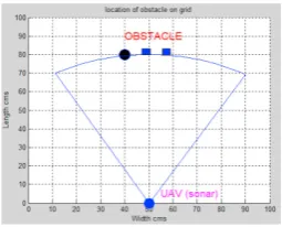
Initial testing was carried with the sensor head mounted on a ground rig. The objective being to determine the location of a 100 mm round pillar within the arc of the transmitter/ receiver at the returned measurement (80 cm) shown in Fig. 7. The dashed lines represent the scan positions of the rotating sonar receivers over a period of 1 second, resulting in 30 samples with each sample containing 2 sub-samples. Note: distance measurement controls the number of samples taken in the time window

Fig.7 Obstacle within sensor field of view

5.1 Test data

(7)

measurement is the distance returned by the combined transmitter / receiver (SRF02). The two sonar receivers (R160) are then rotated with respect to the transmitter / receiver covering the field of view with observations being updated approximately every 100 ms. The scan observations are obtained in the following manner: The scan is divided into 30 segments, during each segment the rising edge of the echo envelope for both received sonar signals are applied to a pair of comparators with a set threshold voltage. The outputs from these comparators provide logic signals which are then combined using an AND operand within a detection window generated by the microcontroller. If both logic signals occur during this window then there is a high probability that the obstacle is at that point in the scan. Echo envelopes for both sonar receivers are then sampled and stored in memory for further analysis within the algorithm. The purpose of this is to only sample data for analysis when there is a high probability that the obstacle may exist at that point in the scan in order to optimise the algorithm. Table 1 shows the output for a typical scan, where ‘1’

[image:7.544.79.442.240.314.2]

represents the probable location of the obstacle with respect to the combined transmitter/receiver. This data is still very noisy and further analysis is needed to localise the area where the obstacle exists within the scan.

Table 1. Partial sample data set

Sample Obstacle? Sample Obstacle?

1 0 16 1

2 0 17 1

3 0 18 0

14 1 29 0

15 0 30 0

Fig. 8 shows the received sonar signals and the rising edge detection window.

[image:7.544.176.344.351.449.2]

Fig. 8 Example of sample data for leading edge signals from both sonar receivers and threshold detection (comparator) point (black dot).

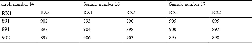
Table 2. Partial sonar envelope sample data set from receivers RX1 and RX2

Sample number 14 Sample number 16 Sample number 17

RX1 RX2 RX1 RX2 RX1 RX2

891 902 893 890 905 895

891 898 904 898 900 892

902 897 906 903 895 890

5.2 Analysis

There are various signal characteristics, or signal metrics, that we can use to analyse discrete-time signals. In this analysis the metrics explored are:

I. Maximum (Peak) frequency (PSD) II. Cross correlation

a. of the raw sampled data

b. of the frequency response data (PSD) III. Energy Spectral Density (PSD)

IV. Power Spectral Density (PSD)

I. The PSD Lomb algorithm is implement using MATLAB for each sub-sample consisting of 20 discrete values. A total of 16 sub-samples (columns of data) is analysed using this method. The first metric to be considered is the maximum frequency for each of the resulting frequency spectra obtained using a peak detector within the window 0- 300 Hz. This is to identify if frequency can be used as a metric for determining the location of the obstacle in the field of view.

I. The PSD output from the Lomb algorithm is shown in Fig. 9a and 9b as an example of sample number 14 data in Table 2.

Fig. 9a Sample 14 (RX1) data and PSD Fig. 9b Sample 14 (RX2) data and PSD

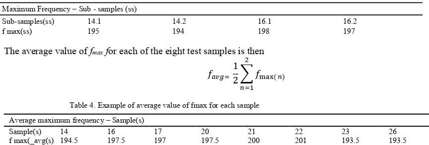
The maximum frequency, fmax at the peak power for each of the resulting frequency spectra using the test data set is shown in Table 3.

Table 3. Example of fmax at maximum power for each sub-sample in the test range 0 – 300 Hz, Maximum Frequency – Sub - samples (ss)

Sub-samples(ss) 14.1 14.2 16.1 16.2

f max(ss) 195 194 198 197

The average value of fmax for each of the eight test samples is then

𝑓𝑓𝑎𝑎𝑎𝑎𝑎𝑎= 1_{2 ∑ 𝑓𝑓}max( 𝑛𝑛) 2

𝑛𝑛=1

Table 4. Example of average value of fmax for each sample Average maximum frequency – Sample(s)

Sample(s) 14 16 17 20 21 22 23 26

f max(_avg(s) 194.5 197.5 197 197.5 200 201 193.5 193.5

From Table 4 it is seen that the change in frequency is not sufficient to deduce anything about the location of the obstacle in the field of view of the sensors.

II. The second metric is Cross correlation this is a means of estimating the degree to which two time series are correlated (Bourke, 2017). Given two time series x (t) and y (t) where i = 0.1, 2, N-1, the cross correlation r, at time delay d is

[image:7.544.41.461.491.564.2]

(8)

I. The PSD Lomb algorithm is implement using MATLAB for each sub-sample consisting of 20 discrete values. A total of 16 sub-samples (columns of data) is analysed using this method. The first metric to be considered is the maximum frequency for each of the resulting frequency spectra obtained using a peak detector within the window 0- 300 Hz. This is to identify if frequency can be used as a metric for determining the location of the obstacle in the field of view.

[image:8.544.56.493.91.296.2]

I. The PSD output from the Lomb algorithm is shown in Fig. 9a and 9b as an example of sample number 14 data in Table 2.

Fig. 9a Sample 14 (RX1) data and PSD Fig. 9b Sample 14 (RX2) data and PSD

The maximum frequency, fmax at the peak power for each of the resulting frequency spectra using the test data set is shown in Table 3.

Table 3. Example of fmax at maximum power for each sub-sample in the test range 0 – 300 Hz, Maximum Frequency – Sub - samples (ss)

Sub-samples(ss) 14.1 14.2 16.1 16.2

f max(ss) 195 194 198 197

The average value of fmax for each of the eight test samples is then

𝑓𝑓𝑎𝑎𝑎𝑎𝑎𝑎= 1_{2 ∑ 𝑓𝑓}max( 𝑛𝑛) 2

[image:8.544.317.478.165.290.2]

𝑛𝑛=1

Table 4. Example of average value of fmax for each sample Average maximum frequency – Sample(s)

Sample(s) 14 16 17 20 21 22 23 26

f max(_avg(s) 194.5 197.5 197 197.5 200 201 193.5 193.5

From Table 4 it is seen that the change in frequency is not sufficient to deduce anything about the location of the obstacle in the field of view of the sensors.

II. The second metric is Cross correlation this is a means of estimating the degree to which two time series are correlated (Bourke, 2017). Given two time series x (t) and y (t) where i = 0.1, 2, N-1, the cross correlation r, at time delay d is

[image:8.544.32.464.367.513.2]

(9)

The cross correlation r (d) raw is obtained using the raw analogue data for each envelope sub-sample representing the

left (RX1) and right sonar (RX2) sensors. Table 5 shows the correlation values and for r (d) raw, and normalised values

[image:9.544.32.466.132.180.2]

to allow plotting of the various metrics on a common graph.

Table 5 .Example of raw analogue data cross correlation between sonar receivers Cross correlation between RX1 and RX2

Sample No. 14 16 17 20

r (d) raw) 0.9944 0.9897 0.9900 0.9918

Normalise 1 0.1696 0.2252 0.5421

The second cross correlation r (d) PSD is obtained using the PSD results for each sub-sample representing the left

[image:9.544.31.461.236.282.2]

(RX1) and right sonar (RX2) sensors. Table 6 shows the results obtained and the normalised values.

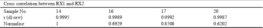
Table 6. Example of PSD data cross correlation between sonar receivers Cross correlation between RX1 and RX2

Sample No. 14 16 17 20

r (d) raw) 0.9995 0.9989 0.9992 0.9987

Normalise 1 0.6929 0.8508 0.6202

III. The third metric is the energy of the PSD sequence which is given by (Corinthios, 2017)

𝐸𝐸 = ∑ |𝑥𝑥(𝑛𝑛)|2

∞

𝑁𝑁=−∞

[image:9.544.30.465.384.419.2]

Where x (n) is the power spectral density data from the Lomb algorithm in the test range 0 to 1500 Hz. Table 7shows the energy content for each of the 16 sub-samples.

Table 7. Example of energy spectral density for each sub-sample PSD signal energy – Sub - samples (ss)

Sub-samples(ss) 14.1 14.2 16.1 16.2

Energy (ss) 1.9017 2.0158 1.7818 1.9402

[image:9.544.31.464.467.503.2]

In order to compare the results with the various metrics the average energy spectral density for each of the samples in Table 8 is obtained by averaging each group of the sub-samples and normalise these values.

Table 8. Example of energy spectral density and normalised values for each sample PSD signal energy – Samples (s)

Sample (s) 14 16 17 20

Energy(s) 3.9205 3.722 4.0492 3.97

IV. The fourth metric is the maximum power for each sub – sample obtained from the power spectral density. This is the maximum power value from the Lomb algorithm in the test range 0 to 1500 Hz, Table 9 shows the power content for each of the sub-samples, with Table 10 the average and normalised values.

Table 9. Example power spectral density for each sample PSD signal power – Sub - samples (ss)

Sub-samples(ss) 14.1 14.2 16.1 16.2

[image:9.544.33.462.633.681.2]

Power (ss) 8.7393 9.9474 8.5218 8.8245

Table 10 Example of power spectral density and normalised values for each sample. PSD signal power – Samples (s)

Sample (s) 14 16 17 20

Energy(s) 17.6867 17.3463 17.9385 17.8487

(10)

[image:10.544.299.427.105.208.2]

Upon examining the four different metrics used in this paper for analysis based on the raw analogue data from the echo sensors and the output from the PSD algorithm, the following can be extrapolated:

Fig. 10 Raw data correlation (Norm (d) raw) Fig. 11 PSD data correlation (Norm (d) PSD)

Fig. 12 Energy spectral density Norm.(s)Energy Fig. 13 Power spectral density Norm.(s)Power

1. The maximum frequency component of the PSD of the returned signal provides no explicit or implicit information to aid in the location of the obstacle within the field of view. All maximum values for each of the samples as shown in Table 4 are in the similar frequency range.

2. The cross correlation of the raw sampled analogue data indicates that the obstacle may exist within two different grid locations (black rectangles) adjacent to the obstacle as shown in Fig. 10. This implies that approximately one third (33%) of the view of the UAV is blocked for flight.

3. The cross correlation of the output data from the PSD algorithm improves the location of the obstacle as shown in Fig. 11 and reduces the blocked area of flight for the UAV to approximately one quarter (25%). 4. In the energy and power spectral density metrics obtained from the PSD algorithm, Fig. 12 and 13 the location of the obstacle is reduced to one grid location reducing the blocked area of flight for the UAV to approximately 1/8 (12.5%).

From these results, it would seem that the most reliable metrics to determine the location of the obstacle based on the test data obtained is the energy and power spectral density. Of these the energy would be first metric to use as it has the lowest standard deviation and average value.

Experiments to date have provided encouraging results. The design of the system is a standalone module with discrete electronics for real time analysis, motorised scanning sensor system and a microcontroller for on board processing. The design would lend itself for use on aerial or ground vehicles with significant improvement in the resolution compared to that of the standard ultrasonic sensor. The standard sensors field of view for obstacle detection

being ± 30°, with the proposed system it should be possible to achieve an improvement where this is reduced to ± 6°.

[image:10.544.83.217.107.206.2] [image:10.544.302.430.252.359.2] [image:10.544.84.218.253.359.2]

(11)

References

Delane, A., Bohórquez, J., Gupta, S. & Schiavenato, M. (2016). Lomb algorithm versus fast fourier transform in heart rate variability analyses of pain in premature infants. In 2016 38th Annual International Conference of the IEEE Engineering in Medicine and Biology Society, EMBC 2016 (Vol. 2016-October, pp. 944-947). [7590857] Institute of Electrical and Electronics Engineers Inc. DOI: 10.1109/EMBC.2016.7590857 Bourke,P. (2017), Cross correlation. Available from: http://paulbourke.net/miscellaneous/correlate/ [Accessed 1st March 2017]

Cassenbrood, B.J. (2006) UAV pose estimation using sonar fusion of sonar and inertial sensors. Traineeship report, Eindhoven University of Technology.

Chen, M.Y., Edwards, D.H. & Boehmer, E.L. (2013) Designing a Spatially Aware and Autonomous Quadcotper. Proceeding of the 2013 IEEE Systems and information, Engineering Design Symposium, University of Virgina, Charlottesville, VA, USA, April 2013

Corinthios, M. (2017), Chapter 12, Energy and Power Spectral Densities. Available from:

http://www.groupes.polymtl.ca/ele2700/docs/Chap12-CorinthBookDraft-final2.pdf [Accessed 2nd May 2017]

Choset, H., Nagatani, H. & Lazar, N. A. (2003) The Arc-transversal median algorithm: A geometric approach to increasing ultrasonic sensor azimuth accuracy, Robotics and Automation, IEEE Transactions on. 19. 513 - 521. DOI: 10.1109/TRA.2003.810580

Devantech Limited (2016), SRF02 Ultrasonic range finder, Available from: http://www.robot-electronics.co.uk/htm/srf02tech.htm, [Accessed 10th January 2006] Drongelen, W. van (2017a, March 10), Scalar Kalman Filter. Available from:

https://epilepsylab.uchicago.edu/sites/epilepsylab.uchicago.edu/files/uploads/Teaching/Kalman%20Filter.pdf [Accessed 10th March 2017a]

Drongelen, W. van (2017b, March 15), Lomb’s Algorithm. Available from: https://www.youtube.com/watch?v=3lP0nKO8nAk [Accessed 15th March 2017b]

Gagelk,N., Muller, T. & Montenegro, S. (2012) Obstacle detection and collision avoidance using ultrasonic distance sensors for an autonomous quadcopters. University of Wurzburg, Germany.

Gageik,N., Benz,P. and Montenegro, S. (2015) Obstacle Detection and Collision Avoidance for a UAV With Complementary Low-Cost Sensors. IEEE Access. 3. 1-1. 10.1109/ACCESS.2015.2432455.

Kodagoda, S., A.S.M. Hemachandra, E., Jayasekara, P., Peiris, R.L., De Silva. & Munasinghe, R. (2006) . Obstacle Detection and Map Building with a Rotating Ultrasonic Range Sensor using Bayesian Combination. Conference: Information and Automation, 2006. ICIA 2006. DO - 10.1109/ICINFA.2006.374159

Murphy,R. (2004) Introduction to AI Robotics. Prentice Hall, India, New Delhi, 2004, pp 210-216