Deciphering satellite observations of compressional ULF waveguide modes

Deciphering satellite observations of compressional

ULF waveguide modes

T. Elsden1_{, A. N. Wright}1_{, and M. D. Hartinger}2

1_{Mathematical Institute, University of St. Andrews, St. Andrews, UK,}2_{Bradley Department of Electrical and Computer}

Engineering, Virginia Polytechnic Institute and State University, Blacksburg, Virginia, USA

Abstract

ULF compressional waveguide modes in Earth’s magnetosphere. In the flank magnetosphere, compressional waves propagate azimuthally but exhibit a mixed standing/propagating nature radially. Understanding this radial dependence will yield information on the energy absorption and transport of these waves. We provide a step by step method that can be applied to observations of flank ULF waves, which separates these fluctuations into incident and reflected parts. As a means of testing, we apply the method to data from a numerical waveguide simulation, which shows the effect on the reflection coefficient when energy is absorbed at a field line resonance.

1. Introduction

Ultralow-frequency (ULF) waves have provided the foundation for a theoretical understanding of the dynam-ics of the magnetosphere since they were first discussed byDungey[1954, 1967]. Subsequently, investigations into the theory of these waves considered the concept of wave coupling between fast and Alfvénic magne-tohydrodynamic (MHD) waves in a cold, ideal plasma [Southwood, 1974;Chen and Hasegawa, 1974]. These works highlighted that the set of field lines on each L shell had its own natural Alfvén frequency. Furthermore, Southwood[1974] examined the singularity occurring at the location where the fast-mode frequency matched the Alfvén frequency, thus developing the concept of field line resonance (FLR). This process describes the transfer of energy from the fast to Alfvénic mode. WhileSouthwood[1974] considered a Cartesian box geom-etry as a model of the dayside magnetopshere,Chen and Hasegawa[1974] discussed the same problem in a dipolar geometry to similar effect.

These studies were followed byKivelson and Southwood[1985, 1986], also using the hydromagnetic box model, where the magnetosphere is treated as a closed cavity. These papers discussed how the large-scale eigenmodes of this magnetospheric cavity could couple to FLRs, which provided an explanation for the observation of selected frequencies being excited by a broadband source. Such eigenmodes are termed global modes and are a standard feature of magnetospheric ULF wave modeling. At the same time, the field of numerical simulations developed rapidly, with many models addressing the problem of FLRs and cavity modes [e.g., Allan et al., 1986a, 1986b;Zhu and Kivelson, 1989;Lee and Lysak, 1989]. The present study, however, is most closely linked to the waveguide model ofRickard and Wright[1994] which expanded on the ideas presented byHarrold and Samson[1992] andSamson et al.[1992]. These works treat the magne-tosphere as an open-ended waveguide as opposed to a closed cavity. This allows for a continuum of wave numbers in azimuth (k_y) and hence a continuum of waveguide frequencies. The authors present further evidence and explanations for the coupling of fast and Alfvénic modes in the terrestrial magnetosphere within the context of a waveguide. The magnetosphere has also been shown to behave as a waveguide in global MHD simulations [Claudepierre et al., 2016], giving further support to its use here.

The above concepts and references regarding ULF waves are introduced as they underpin the theory of this work. We present analytical and numerical models to study ULF waveguide modes in the flank mag-netosphere. Our aim is to demonstrate a procedure that can subsequently be used in conjunction with observations. Compressional waveguide modes propagate azimuthally on the flanks but have a mixed stand-ing/propagating nature in the radial direction. We decompose these fluctuations into radially propagating inward (incident) and outward (reflected) waves, which can provide information on energy transport and absorption in the flank magnetosphere. The analysis requires signals whose amplitudes do not vary drastically

TECHNICAL

REPORTS:

METHODS

Key Points:

• Derive a method for estimating incident and reflection coefficients for flank ULF waveguide modes • Test method on simulation data which

provide consistent results • Method will be applied to satellite

data in the future

Correspondence to:

T. Elsden,

te55@st-andrews.ac.uk

Citation:

Elsden, T., A. N. Wright, and M. D. Hartinger (2016), Deciphering satellite observations of compres-sional ULF waveguide modes,

J. Geophys. Res. Space Physics,

121, doi:10.1002/2016JA022351.

Received 10 JAN 2016 Accepted 15 MAR 2016

Accepted article online 21 MAR 2016

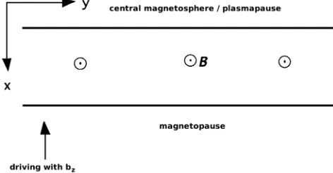
Figure 1.A schematic of the model magnetospheric waveguide. The magnetopause boundary is driven as indicated, launching waves propagating iny(azimuthally).

over one or two periods and that have a well defined frequency. Space-based observations of such ULF waves have been reported byRae et al.[2005],Eriksson et al.[2006],Clausen et al.[2008],Hartinger et al.[2011], and Hartinger et al.[2012]. We apply our method of deriving these coefficients to simulated data, as a means of validating the procedure, with the aim of applications to real data in the future.

While methods exist for the routine identification and characterization of cavity modes in satellite obser-vations [e.g., Waters et al., 2002], there are no comparable techniques for waveguide modes. This adds uncertainty to waveguide/global mode observational studies. For example, in a statistical study estimating global mode occurrence rates outside the plasmasphere,Hartinger et al.[2013] identified potential global modes using cavity mode selection criteria: globally coherent, monochromatic fast-mode waves with elec-tric/magnetic perturbations consistent with radially standing waves. As discussed byHartinger et al.[2013], these criteria excluded tailward propagating waveguide modes, likely biasing noon occurrence rates higher than flank rates and leading to an unrealistically low overall global mode occurrence rate.

The paper is organized as follows: section 2 outlines the model geometry and the equations for the problem then discusses the steps to follow to perform the analytic method used for deriving the incident and reflection coefficients. Section 3 discusses the application of our analytical model to simulated data. Here the numerical method and signal processing techniques employed are mentioned in detail. Concluding remarks are given in section 4, and a full derivation of the procedure and reference equations are provided in AppendixA.

2. Theory and Model

2.1. Waveguide Geometry

The Cartesian hydromagnetic box model has been extensively used to study the behavior of ULF wave modes in the flank magnetosphere [e.g.,Southwood, 1974;Kivelson and Southwood, 1985, 1986].x̂ is taken as the radial direction, positive outward.ŷrepresents the azimuthal direction, with the antisunward direction being aligned with positive/negativeŷon the dusk/dawn flank, respectively.ẑis in the direction of the background magnetic field taken asB=B₀ẑ. Figure 1 gives a representation of this waveguide.

The plasma is assumed to be cold (low𝛽) and ideal. The waveguide has a perfectly reflecting inner boundary inxmodeling some natural boundary in space such as the plasmapause or a turning point while the outer boundary (magnetopause) is driven. We consider only fundamental standing modes in thezdirection, where field lines are fixed at their ionospheric footpoints by assuming nodes of velocity there. This reduces the com-putational model to a two-dimensional waveguide allowing for faster computation and better resolution. The magnetic equator is placed atz=0, and the single Fourier mode inzis expressed for each of the components asux,uy,bz∼ cos(kzz)andbx,by∼sin(kzz). This assumption is used in the component definitions given in section 2.2. The inhomogeneity of the plasma is characterized by allowing the density to vary with radius (x). In the numerical simulations we normalize the equations to deal with dimensionless quantities, but for the analytical method we use the dimensional linearized MHD equations which can be expressed as

𝜕b_x

𝜕t =B0

𝜕u_x

𝜕z, (1)

𝜕by

𝜕t =B0

𝜕uy

𝜕b_z

𝜕t = −B0

(_𝜕u

x

𝜕x +

𝜕u_y 𝜕y

)

, (3)

𝜕u_x

𝜕t =

V2 A B0

(_𝜕b

x

𝜕z −

𝜕b_z 𝜕x

)

, (4)

𝜕uy

𝜕t =

V2 A B₀

(_𝜕b

y

𝜕z −

𝜕bz

𝜕y )

, (5)

whereVAis the Alfvén speed andB0the background magnetic field strength. For the analytic work in this paper, we assume the lowest-order WKB approximation to the above equations (1)–(5). Analysis of this type is discussed in detail in, for example,Inhester[1987] andWright[1994]. This gives the radial wave numberkxas

k_x2(x) = 𝜔

2

V2 A(x)

−k_y2−k2_z, (6)

with the phase inxdefined as

Φ_x(x) =

∫

x

kx(x′)dx′. (7)

2.2. Tailward Traveling Wave Model

As mentioned previously, the goal of this study is to understand the dynamics of tailward traveling waves that exhibit a mixed propagating and standing nature radially. In this regard consider a wave of the form

bx=Aicos

(

kyy− Φx−𝜔t

)

sin(kzz) +Arcos

(

kyy+ Φx−𝜔t

)

sin(kzz). (8)

A_idenotes the incident coefficient andA_rthe reflected, both with units of tesla. This stems from inward prop-agation being in the negativex̂direction.k_x,k_y, andk_zare the wave numbers;x,y, andzare the positions in thex̂,ŷ, andẑdirections, respectively. We choose to define theb_xcomponent purely as a start point from which to derive the other component forms. Using equations (1)–(5) yields

b_y= −A_iky kx

cos(k_yy− Φ_x−𝜔t)sin(k_zz) +A_rky kx

cos(k_yy+ Φ_x−𝜔t)sin(k_zz). (9)

b_z= −Aikz

kx

{ 1− 𝜔

2

V2 Ak2z

}

sin(k_yy− Φ_x−𝜔t)cos(k_zz)

+Arkz

kx

{ 1− 𝜔

2

V2 Ak2z

}

sin(k_yy+ Φ_x−𝜔t)cos(k_zz).

(10)

ux= − Ai B₀

𝜔 k_zsin

(

kyy− Φx−𝜔t

) cos(kzz)

− Ar

B0 𝜔 kz

sin(kyy+ Φx−𝜔t

) cos(kzz).

(11)

uy= Ai B₀

𝜔ky k_xk_zsin

(

kyy− Φx−𝜔t

) cos(kzz)

− Ar

B0 𝜔ky kxkz

sin(k_yy+ Φ_x−𝜔t)cos(k_zz).

(12)

ky,kz,Φx, andkzz. The position inyis not required since the model assumes that the wave is propagating in theŷdirection. Hence, changingymerely shifts the phase of the entire solution and is similar to moving the time origin but does not affect any of the quantities listed above. Not all of the quantities provided from satellite data are independent, which reduces the number of “knowns.” These independent quantities are the amplitudes ofb_x,b_y,b_zandu_x, the frequency𝜔, the local Alfvén speedV_A, and the phase shift betweenb_xand b_y, denoted by𝜙. Stipulating−𝜋 < 𝜙≤𝜋,𝜙is positive ifb_yleadsb_xby less than𝜋and negative ifb_ytrailsb_x by less than𝜋.u_yis not an independent quantity as it can be expressed in terms of the amplitudes ofu_x,b_x, andb_y. Equally, any of these quantities could have been removed instead, in favor ofu_y.

To proceed with determining the unknowns, it is useful to express the components in terms of a single amplitude and phase for the purpose of comparison to data. For example, we expressbxas

bx=b̄xcos(𝜓1−𝜔t), (13)

whereb̄xis the amplitude and𝜓1a phase shift. Considering this for all components, we can then equate the two expressions for each component, e.g., (8) and (13). This allows the expression of the amplitudes in terms of the incident and reflection coefficients. After some algebra we derive the following system of equations:

̄ bx= ±

√ A2

i +A2r +2AiArcos(2Φx)sin(kzz), (14)

̄ by= ±

ky k_x

√ A2

i +A2r −2AiArcos(2Φx)sin(kzz), (15)

̄ bz= ±

kz k_x

{ 𝜔2 V2

Akz2

−1 }√

A2

i +A2r−2AiArcos(2Φx)cos(kzz), (16)

̄ ux= ±_B𝜔

0kz

√ A2

i +A2r +2AiArcos(2Φx)cos(kzz), (17)

tan(𝜙) = 2AiArsin

( 2Φ_x)

A2 r −A

2 i

, (18)

𝜔2 V2 A

=k2_x(x) +k_y2+k2_z, (19)

where as mentioned above,b̄_x,b̄_y,b̄_z, andū_xare the amplitudes ofb_x,b_y,b_z, andu_x, respectively, and we restate the WKB fast-mode dispersion relation from (6) as (19). This system contains six equations for the seven unknowns previously listed. It is therefore necessary to infer one more piece of information from the satellite data. Multiple satellite missions and ground-based observations have the capability of estimat-ing one of the wave numbers. For example, phase differences between signals measured at longitudinally spaced satellites or ground stations can be used to obtainky[e.g.,Mathie and Mann, 2000;Sarris et al., 2013] and phase differences between signals measured at multiple locations on the same field line can be used to obtainkz[e.g.,Takahashi et al., 1987]. Once a component of the wave vector has been estimated, (14)–(19) may then be solved.

2.3. Solution Method

Figure 2.Variation of the Alfvén speed profile with radius (x) given by equations (20) and (21), adapted fromWright and Rickard[1995b]. The plotted curves correspond to the values

x₀=0.95,1.0,1.2,1.4,1.6,1.8, with the first and last annotated. The dashed line represents the value ofx_c=0.8.

2.3.1.kzMeasured

1. Use (A3) to findky, choosing the positive root for an observation in the dusk flank and the negative root for the dawn flank.

2. Use (A4) to findkx(x).

2.3.2.kyMeasured

1. Use (A5) to findkz, taking the positive root. 2. Use (A4) to findkx(x).

2.3.3.k_xMeasured

1. (A7) and (A8) together determine four values forky. Take the two positive values for a dusk flank observation and the two negative values for the dawn flank.

2. Use (A9) to find the correspondingkzvalue.

2.3.4. DeterminingAiandAr

After completing steps 1 and 2 for one of the cases above, proceed to the steps below to determineAiandAr.

1. Use (A2) to findk_zz. Choose the positive sign for an observation above the magnetic equator (z>0) and the negative sign for an observation below (z<0).

2. Givenk_zz, determine the coefficientsCandDfrom the first equalities in (A10) and (A11) andPandQfrom (A19) and (A20), respectively.

3. UsingPandQin (A18) defines two values forA2

i and hence four solutions forAi. 4. (A21) yields two values ofArfor eachAi, giving eight solution pairs ofAiandAr.

5. (A24) and (A25), with (A23), define four values ofΦ(x)for eachAiandArcombination, which implies a total of 32 solution combinations.

Following the above systematic approach, all possible solutions can be determined. To eliminate the spurious solutions, the component time series are formed using equations (8)–(12) and are then compared to the data to see which ones match. It is this procedure which is followed in the next section.

3. Method Testing—Simulation Case Study

We now demonstrate how to test the above analytical method for determining incident and reflection coefficients on simulated data. This will establish the reliability of the method on numerical data before attempting to apply the method to satellite data. The following subsections outline the details of the simula-tion, how to generate appropriate signals to input to the method through signal analysis, and the final results demonstrating the use of the method.

3.1. Numerical Model

Equations (1)–(5) are solved numerically using a leapfrog-trapezoidal algorithm [Rickard and Wright, 1994]. We first normalize the magnetic field by the background field strengthB₀, the density by that at the inner boundary𝜌(0), and the length by the width of the waveguide inx. FollowingWright and Rickard[1995b], we adopt a variation in the Alfvén speed of the form

VA(x) =1− x x0

, 0<x≤xc (20)

V_A(x) =

x0 (

1−xc

x0

)3( 1−xc

) (

x0−2xc+1

) ( 1−xc

)

− (1−x)2, xc<x<1 (21)

The waveguide has a radial extent of 1 which corresponds to a physical length of 10R_E. The length inyvaries for the different simulations dependent on the wavelength. We choose an appropriate spatial resolution of the grid, time step, and total length of simulation to satisfy the Courant-Friedrichs-Lewy condition and resolve the phase mixing length. Typically, energy is conserved to one part in 105_{or better.}

To model tailward traveling waves, we drive the system with a running disturbance on the magnetopause, more details of which are given in the results section 3.3. The magnetopause boundary is driven by pertur-bations in thezcomponent of the magnetic field,b_z. This has been demonstrated as an effective means of modeling driving by magnetic pressure [Elsden and Wright, 2015]. Furthermore, given a perfectly reflecting inner boundary, driving in this way allows the fundamental radial mode to be a quarter wavelength mode. This lowers the natural waveguide eigenfrequencies, bringing them more in line with the observed frequencies without resorting to an unphysical plasma density [Mann et al., 1999].

To efficiently model an open-ended waveguide iny, we introduce dissipation regions at either end (beyond the region of interest), which act to absorb any perturbations as if they had run out of the waveguide. This is implemented by adding a linear drag term to the equation of motion in these regions, the amplitude of which can be adjusted as per the strength of dissipation required.

3.2. Signal Generation and Analysis

Our procedure is appropriate for signals that are purely propagating in theydirection. The signal has to be relatively monochromatic and cannot display a great variation in amplitude over one period. To produce such a signal from our simulations, we drive the outer boundary with a tailward traveling wave packet, an exam-ple of which will be given in section 3.3. Our control lies with the amplitude, wavelength, phase speed, and number of cycles in the packet.

To model a satellite observation, we pick a location in the waveguide and consider the time series of the components. These signals are band pass filtered using an Interactive Data Language filtering routine, in a similar manner to the filtering of observational data. For our procedure we require the amplitudes of the components and the phase shift betweenb_xandb_y, as discussed in section 2.2. To derive these from the simulation data, we use an analytic signal method over the desired time interval, which has been used in observations by, for example,Glassmeier[1980] andHartinger et al.[2011]. The analytic signals_a(t)is a complex valued function formed from the real signals(t)and its Hilbert transformŝ(t)as

s_a(t) =s(t) +iŝ. (22)

This removes any negative frequency contributions to the signal. In this form the instantaneous phase of each signal,𝜓, is determined by

𝜓=tan−1

( ̂ s(t)

s(t)

)

, (23)

and hence, we can calculate the required phase shift between theb_x andb_ycomponents. The amplitude envelope for the signal is determined from

|sa(t)|=

√

s(t)2₊̂_s(t)2_{, (24)}

which is averaged over the cycles considered to determine their amplitude. This then yields all the required information to determine the incident and reflection coefficients.

Figure 3.(top) Temporal variation of the perturbationb_zon the driven magnetopause boundary (x=1), in the center of the driven section. (bottom) Spatial variation in azimuth ofbzon the driven magnetopause boundary, at timet=45.

The vertical dashed lines represent the start of the dissipation regions (y<−5,y>5), where the boundary is not driven.

Figure 5.FFT power spectrum of the unfilteredb_zsignal at locationsx=0_.9,y=0, andz=0_.5, showing a

dimensionless cyclic frequency of 0.23 corresponding to the driving frequency.

kz is taken to be 𝜋∕2 in dimensionless units (corresponding to a dimensional field line length of 20RE), and the parameter controlling the gra-dient of the Alfvén speed profile,x0, is set to 2.7, such that the FLR continuum does not overlap any of theky =0waveguide eigenfrequencies as men-tioned above. The other parameter in the Alfvén speed definition ((20) and (21)),xc, is chosen as 0.8. We choose to excite an Alfvén resonance in the guide atxr = 0.2, by setting the driving frequency equal to the Alfvén frequency at this location. This yields a dimensionless angular driving frequency of 𝜔r=1.4544.kyvaries between each simulation and will control the efficiency of the coupling between the fast and Alfvénic modes. The modes are decou-pled in theky → 0andky → ∞limits, and hence, we expect the strongest coupling for moderateky values [Kivelson and Southwood, 1986]. The maximumky is determined such that the mode is oscillatory (not evanescent) inxat the satellite location. The driving frequency is held constant between the different simulations by varying the phase speed of the driver accordingly.

Before stating the results, we list a step by step view of the method for clarity.

1. Specify a wavelength and phase speed for the magnetopause driver then run the simulation.

2. Choose the satellite location on the magnetopause side of the resonance, retrieve component time series. 3. Band pass filter the data around the driving frequency.

4. Use the analytic signal method to determine instantaneous phase and amplitude. 5. Derive all possible solution combinations forAi,Arvalues, as per section 2.3.

6. Select correct solutions by reconstructing the signal usingAiandArand comparing to the simulation signal.

3.3. Results

One of the simulation runs for a specific value ofk_ywill be discussed to demonstrate the method. For the equilibrium parameters described above the value ofk_ycan vary over 0≤k_y≤1.503, the upper bound being determined by maintaining an oscillatory nature inxat the magnetopause. An example of the temporal and spatial dependence of the magnetopause driver is given in Figure 3, for the casek_y=1.4. Note that the spatial form of the driving condition is a sine wave that travels in theydirection at a speed𝜔∕k_yand is nonzero over the window−5<y<5in this example. The frequency𝜔is chosen to match the Alfvén frequency atx_r=0.2; hence, these parameters determine the azimuthal phase speed of the magnetopause driver we impose. We select a location in the waveguide for the model satellite ofx=0.9,y=0, andz=0.5. The position is chosen close to the magnetopause boundary such that the mode is oscillatory and not evanescent inx.

Figure 6.Time series ofb_y(black) andu_y(red) at the Alfvén resonance locationx=0.2, withy=0.

Figure 7.Time series interval fromt=28.5tot=36.0ofb_x(black) andb_y(red) showing (top) the unfiltered data (solid) with the band-pass filtered data (dashed); (middle) filtered data (solid) with phase and amplitude averaged signal (dashed), vertical dashed lines indicate the phase shift𝜙; and (bottom) phase and amplitude averaged data (solid), reconstructed signal fromAiandArvalues (dashed, which overlies the solid line exactly in this example). The dotted

lines represent a spurious solution that does not reproduce the desired (solid line) signals, so is discarded.

waveguide interior. The monochromatic nature of the signal is confirmed by considering the fast Fourier trans-form (FFT) power spectra, displayed in Figure 5 forbzat the satellite location. The angular driving frequency of 1.4544 is reproduced as a cyclic frequency of 0.23.

To check that a resonance is being excited at the appropriate location, we check the behavior of the transverse magnetic field and velocity components. Figure 6 shows the secular growth in time of these components, which is expected for a steadily driven resonance in the absence of dissipation.

The next step is to band-pass filter the data for the desired frequency. Considering the idealized case that we present here, the effect of filtering is not drastic but still is a worthwhile procedure to demonstrate how our method would be applied to a real data signal. A small time interval covering one to two periods is recon-structed from the signal filtered over cyclic frequencies from 0.17 to 0.29. Figure 7 (top) displays the unfiltered and filtered signals.

Figure 8.The ratioAr∕Aiplotted againstkyfor 21 different

k_yvalues.

discussion on choosing 𝜙). Since the filtered signal is already of near-constant amplitude and frequency, the dashed line representing the signal constructed from the instantaneous phase and average amplitude lies almost directly on top. All of the knowns are now determined, and the system can be solved as described in section 2.3. This yields the incident and reflection coefficients AiandAr. For the simulation in question, the abso-lute value of these coefficients was determined as |Ai|=1.202and|Ar|=1.112. These correct solutions are found by matching the signal components reconstructed from the derived quantities as per (8)–(12), with the phase and amplitude averaged signal. Figure 7 (bottom) displays these signals for thebx(black) andby(red) components. The dotted lines represent a reconstructed solution that does not match the solid lines so represents a spurious solution that we shall discard. The dashed lines are barely vis-ible as they lie directly on top of the original signal, which confirms the values ofA_iandA_rused to produce them corresponding to the correct roots.

Furthermore, the correct values are in line with our original prediction that the reflection coefficient will be smaller than the incident due to energy lost from the fast mode at the resonance. The amount of energy deposited and hence the ratio of the reflected to incident coefficients are dependent on the efficiency of the wave coupling, which is controlled byky. Ifkyis small, the gradients ofbzin theŷdirection which drive the resonance become small and hence the coupling is weak. For largeky, the turning point of the mode retreats from the resonance toward the magnetopause boundary, and the amplitude decays evanescently, meaning that the fast mode does not penetrate to the resonance location. This behavior produces a classic curve of absorption againstky[seeKivelson and Southwood, 1986, Figure 2 ]. As a test of the values produced forAiand Ar, we ran several simulations for different values ofky, performed the same analysis as above, and plotted the resulting ratio ofArtoAi. This is displayed in Figure 8. A clear trend appears showing the ratio tending to one where little energy is transferred to the resonance (as in theky=1.4case above), while in regions where the coupling is more efficient, the ratio drops considerably. This is further confirmation that the method employed to determine the incident and reflection coefficients is behaving consistently.

4. Conclusions

In this work we have introduced a method for determining incident and reflection coefficients for flank ULF waveguide modes. This method is valid for tailward traveling waves of roughly constant amplitude with a clearly defined frequency. Despite seeming like an idealized case, observations of such signals have been recently published [Rae et al., 2005;Eriksson et al., 2006;Clausen et al., 2008;Hartinger et al., 2011, 2012]. The coefficients derived are correlated with the energy absorption of the magnetospheric interior, as demon-strated by the lowering of the reflection coefficient when energy is absorbed at a FLR. The method produces consistent results, reproducing a similar resonant absorption curve to that ofKivelson and Southwood[1986], showing the change in the efficiency of wave coupling with azimuthal wave number. Since the only require-ments of the method are a set of time series together with certain amplitudes and phase shifts, this technique could also be applied to results from a global MHD simulation. Evidently, the Cartesian geometry used in our modeling is a simplification. Future studies could employ spatial eigenmodes based upon a realistic magne-tospheric equilibrium and so improve the accuracy of our technique when applied to satellite data or results from global magnetospheric simulations. The overall purpose of this work has been to test the method on simulation data in preparation for using it with satellite observations of flank ULF compressional modes in the future.

Appendix A: Solution Method

the frequency𝜔, the Alfvén speedV_A, and the phase difference betweenb_yandb_x, denoted by𝜙(refer to section 2.3 for full details on𝜙). As discussed at the end of section 2.2, one of the wave numbers is also required to solve the system. In each of the sections below, we discuss the different approaches depending on which wave number is estimated most accurately. First, however, we must resolve the choices of signs in equations (14)–(19). Since it is the amplitudes of the components (denoted by an overscore) that are being used, the expressions for these amplitudes must be positive. Hence, the choice of sign is dependent on the signs of sin(kzz)and cos(kzz). For a fundamental mode in theẑdirection,−𝜋∕2 < kzz < 𝜋∕2. cos(kzz)is positive over the range ofkzz, and hence, the signs in equations (16) and (17) are taken to be positive. If the observation is taken below the magnetic equator,zis less than zero, which implies sin(kzz) < 0and hence we choose negative signs for equations (14) and (15) such that the amplitudes remain positive. Equally, if the satellite is above the magnetic equator, positive signs are taken in these equations.

There is one exception to this which occurs whenkyis negative, sincekyappears as a coefficient in (15). If the observation is in the dusk flank, takekyto be positive, and if the observation is in the dawn flank, takekyto be negative. This stems from the positiveŷdirection being tailward in the dusk flank. Therefore, in the situa-tion wherekyis negative, the above sign choices must be reversed for equation (15) such that the amplitude remains positive.

A1.kzMeasured

To begin with, consider the case wherekz, the field-aligned wave number, is known from observations. To find the positionz, we divide (14) by (17) to give

tan(kzz) = ±

𝜔 ̄b_x k_zū_x

1

B₀ (A1)

⇒kzz=tan−1

(

±𝜔 ̄bx

kzūx 1 B0

)

, (A2)

where the sign choice is determined from the position inzabove or below the magnetic equator (positive if z>0).k_ycan be determined from the ratio of (16) to (15), substituting for tan(k_zz)using (A1) to give

̄ bz

̄ by

= ± B0

𝜔ky

( 𝜔2 V2 A

−k2 z

) ̄ ux

̄ bx

,

⇒k_y= ± ūx

̄ b_y ̄ bxb̄z

B₀ 𝜔

( 𝜔2 V2 A

−k2 z

) ,

(A3)

where the plus/minus root is taken for observations on the dusk/dawn flank.kx(x)can now be determined from the fast-mode dispersion relation (6) as

k_x(x) =

√ 𝜔2 V2 A

−k2

y−kz2, (A4)

wherekx(x)is taken to be positive (inward and outward propagation inxis accommodated in the definition ofbxin equation (8)). At this point,kzz,ky, andkx(x)are known and we can proceed to section A4 to calculate A_iandA_r.

A2.kyMeasured

If insteadky, the azimuthal wave number, is provided by satellite data, we proceed in a similar manner to the above forkz. Rearranging (A3) gives

kz=

√ √ √ √𝜔2

V2 A

−|ky|_B𝜔 0

̄ bxb̄z

̄ uxb̄y

. (A5)

A3.k_xMeasured

The case wherek_x, the radial wave number, is provided from observations is not so straightforward as we lack an expression for one of the other wave numbers in terms ofk_xalone. We proceed by rewriting (A3) using (A4) as

k_y= ±ūx

̄ b_y ̄ bxb̄z

B₀ 𝜔 (

k2 x(x) +k

2 y

)

. (A6)

Again, the sign fork_y is determined as being positive on the dusk flank and negative on the dawn flank. Rearranging (A6) as a quadratic forkyand solving yields

k_y= ±X

2± √

X2 4 −kx(x)

2_{, (A7)}

where

X= b̄xb̄z

̄ uxb̄y

𝜔 B0

. (A8)

Forky>0choose the first sign to be positive, while forky<0choose the first sign to be negative. The second sign choice represents two distinct solutions which have to be carried through the procedure until they can be tested for their validity. This doubles the total number of possible solutions, and indeed, each of the above k_yvalues can lead to a correct solution. For this reason, it is preferable for the azimuthal or field-aligned wave numbers to be provided instead of the radial wave number, as for these cases a single solution can always be determined. Once the values ofk_yhave been calculated, the correspondingk_zvalues are determined from the fast-mode dispersion relation as

kz=

√ 𝜔2 V2 A

−k2

y−k2x(x), (A9)

and then the values ofk_zzare found from (A2). Now that the wave numbers are known, proceed to section A4. A4. DeterminingAiandAr

The above steps outline how to determine the wave numbers depending on which is provided by the obser-vation. The following working shows how then to calculate the incident and reflection coefficientsAiandAr given the wave numbers. We begin by squaring (14) and (15) then adding and subtracting to give

C=b̄x 2 +k 2 x k2 y ̄ by 2

=2(A2 i +A

2 r

) sin2_(k

zz), (A10)

D=b̄x 2 −k 2 x k2 y ̄ by 2

=4AiArcos(2Φx)sin2(kzz). (A11)

We attempt to form the terms on the right-hand side of (18). The denominator can be written using (A10), as A2_r−A2_i =A_r2+A2_i −2A2_i = C

2 sin2_(k zz)

−2A2_i. (A12)

The numerator can be formed using (A11) as

2A_iA_rsin(2Φ_x) = ±1

2 √

16A2 iA2r −

D2 sin4(kzz)

. (A13)

Using (A12) and (A13) in (18) gives

tan(𝜙) = ±1

2 √

16A2 iA2r −

D2

sin4_(k zz)

C 2 sin2_(k

zz)

−2A2 i

, (A14)

⇒tan2(𝜙)

( C 2 sin2_(k

zz)

−2A2_i )2

= 1

4 (

16A2_iA2_r− D

2

sin4_(k zz)

)

The goal is to eliminateA_rin terms ofA_i. Expanding brackets and replacingA2

rusing a rearrangement of (A12), we arrive at a fourth-order equation forA_ias

A4 i −

C 2 sin2_(k

zz) A2

i +

C2_sin2_𝜙+D2_cos2_𝜙 16 sin4_(k

zz)

=0. (A16)

The above equation can be written as

A4 i −PA

2

i +Q=0, (A17)

⇒A2 i =

P 2±

1 2

√

P2_−4Q, _(A18)

where

P= C

2 sin2_(k zz)

, (A19)

Q= C

2_sin2_𝜙+D2_cos2_𝜙 16 sin4_(k

zz)

. (A20)

(A18) defines four solutions forAi givenC,D,P, andQ. Through squaring, spurious roots will have been introduced that will be discarded at the end.Aris found from rearranging (A12) as

A_r= ±

√ P−A2

i. (A21)

This implies that there are eight possible combinations ofAiandArvalues. Each of these combinations can then be used to calculate the WKB phaseΦ_x. Rearranging (14) gives

2A_iA_rcos(2Φ_x) = b̄x

2

sin2(kzz)

−A2 i −A

2

r, (A22)

Φ_x= 1

2cos

−1 {

1 2A_iA_r

( ̄ bx

2

sin2_(k zz)

−A2_i −A2_r )}

. (A23)

Taking the inverse cosine results in four solutions forΦ_x, which can be expressed as

Φ_x= 1

2cos

−1_{(𝛼) +n𝜋,n=0,1, (A24)}

Φ_x=1

2 (

2𝜋−cos−1_(𝛼))_{+n𝜋, n=0,1, (A25)}

where𝛼is the curly bracketed term in (A23) and cos−1_{lies between 0 and𝜋. Thus, with four solutions forΦ} x(x) and eight combinations ofAiandAr, there are 32 possible solutions. The correct solutions are determined by constructing the components given in (8)–(12) using the derived values ofAi,Ar, etc., then checking these signals against the data. The solutions associated with the spurious roots acquired during the calculation may be identified and disregarded as the reconstructed signals will not match the original ones. This procedure will leave four valid combinations, one for each of the arbitrary phase choices in (A24) and (A25). Any one of these solutions may be used unless additional information is available to identify a particular solution as being more appropriate.

References

Allan, W., E. M. Poulter, and S. P. White (1986a), Impulse-excited hydromagnetic cavity and field-line resonances in the magnetosphere,

Planet. Space Sci.,34(4), 371–385, doi:10.1016/0032-0633(86)90144-3.

Allan, W., E. M. Poulter, and S. P. White (1986b), Hydromagnetic wave coupling in the magnetosphere–Plasmapause effects on impulse-excited resonances,Planet. Space Sci.,34(12), 1189–1200, doi:10.1016/0032-0633(86)90056-5.

Chen, L., and A. Hasegawa (1974), A theory of long-period magnetic pulsations: 1. Steady state excitation of field line resonance,J. Geophys. Res.,79(7), 1024–1032, doi:10.1029/JA079i007p01024.

Acknowledgments

Claudepierre, S. G., F. R. Toffoletto, and M. Wiltberger (2016), Global MHD modeling of resonant ULF waves: Simulations with and without a plasmasphere,J. Geophys. Res. Space Physics,121, 227–244, doi:10.1002/2015JA022048.

Clausen, L. B. N., T. K. Yeoman, R. Behlke, and E. A. Lucek (2008), Multi-instrument observations of a large scale Pc4 pulsation,Ann. Geophys.,

26, 185–199, doi:10.5194/angeo-26-185-2008.

Dungey, J. W. (1954), Electrodynamics of the outer atmosphere,Sci. Rep. No. 69.,Pennislavania State Univ., lonos, Res. Lab., State College, Pa. Dungey, J. W. (1967), Hydromagnetic waves, inPhysics of Geomagnetic Phenomena, vol. 2, edited by S. Matsushita and W. H. Campbell,

pp. 913–934, Academic, San Diego, Calif.

Elsden, T., and A. N. Wright (2015), The use of the Poynting vector in interpreting ULF waves in magnetospheric waveguides,J. Geophys. Res. Space Physics,120, 166–186, doi:10.1002/2014JA020748.

Eriksson, P. T. I., L. G. Bloomberg, S. Schaefer, and K.-H. Glassmeier (2006), On the excitation of ULF waves by solar wind pressure enhancements,Ann. Geophys.,24, 3161–3172, doi:10.5194/angeo-24-3161-2006.

Glassmeier, K. H. (1980), Magnetometer array observations of a giant pulsation event,J. Geophys.,48(3), 127–138.

Harrold, B. G., and J. C. Samson (1992), Standing ULF modes of the magnetosphere: A theory,Geophys. Res. Lett.,19, 1811–1814, doi:10.1029/92GL01802.

Hartinger, M., V. Angelopoulos, M. B. Moldwin, K.-H. Glassmeier, and Y. Nishimura (2011), Global energy transfer during a magnetospheric field line resonance,Geophys. Res. Lett.,38, L12101, doi:10.1029/2011GL047846.

Hartinger, M., V. Angelopoulos, M. B. Moldwin, Y. Nishimura, D. L. Turner, K.-H. Glassmeier, M. G. Kivelson, J. Matzka, and C. Stolle (2012), Observations of a Pc5 global (cavity/waveguide) mode outside the plasmasphere by THEMIS,J. Geophys. Res.,117, A06202, doi:10.1029/2011JA017266.

Hartinger, M. D., V. Angelopoulos, M. B. Moldwin, K. Takahashi, and L. B. N. Clausen (2013), Statistical study of global modes outside the plasmasphere,J. Geophys. Res. Space Physics,118, 804–822, doi:10.1002/jgra.50140.

Inhester, B. (1987), Numerical modeling of hydromagnetic wave coupling in the magnetosphere,J. Geophys. Res.,92(A5), 4751–4756, doi:10.1029/JA092iA05p04751.

Kivelson, M. G., and D. J. Southwood (1985), Resonant ULF waves: A new interpretation,Geophys. Res. Lett.,12(1), 49–52, doi:10.1029/GL012i001p00049.

Kivelson, M. G., and D. J. Southwood (1986), Coupling of global magnetospheric MHD eigenmodes to field line resonances,J. Geophys. Res.,

91(A4), 4345–4351, doi:10.1029/JA091iA04p04345.

Lee, D. H., and R. L. Lysak (1989), Magnetospheric ULF wave coupling in the dipole model: The impulsive excitation,J. Geophys. Res.,94(A12), 17,097–17,103, doi:10.1029/JA094iA12p17097.

Mann, I. R., A. N. Wright, K. J. Mills, and V. M. Nakariakov (1999), Excitation of magnetospheric waveguide modes by magnetosheath flows,

J. Geophys. Res.,104(A1), 333–353, doi:10.1029/1998JA900026.

Mathie, R. A., and I. R. Mann (2000), Observations of Pc5 field line resonance azimuthal phase speeds: A diagnostic of their excitation mechanism,J. Geophys. Res.,105, 10,713–10,728, doi:10.1029/1999JA000174.

Rae, I. J., et al. (2005), Evolution and characteristics of global Pc5 ULF waves during a high speed solar wind speed interval,J. Geophys. Res. Space Physics,110, A12211, doi:10.1029/2005JA011007.

Rickard, G. J., and A. N. Wright (1994), Alfvén resonance excitation and fast wave propagation in magnetospheric waveguides,J. Geophys. Res.,99(A7), 13,455–13,464, doi:10.1029/94JA00674.

Samson, J. C., B. G. Harrold, J. M. Ruohoniemi, and A. D. M. Walker (1992), Field line resonances associated with MHD waveguides in the magnetosphere,Geophys. Res. Lett.,19(5), 441–444, doi:10.1029/92GL00116.

Sarris, T. E., X. Li, W. Liu, E. Argyriadis, A. Boudouridis, and R. Ergun (2013), Mode number calculations of ULF field-line resonances using ground magnetometers and THEMIS measurements,J. Geophys. Res. Space Physics,118, 6986–6997, doi:10.1002/2012JA018307. Southwood, D. J. (1974), Some features of field line resonances in the magnetosphere,Plante. Space Sci.,22(3), 483–491,

doi:10.1016/0032-0633(74)90078-6.

Takahashi, K., J. F. Fennell, E. Amata, and P. R. Higbee (1987), Field-aligned structure of the storm time Pc 5 Wave of November 14–15, 1979,

J. Geophys. Res.,92, 5857–5864, doi:10.1029/JA092iA06p05857.

Waters, C. L., K. Takahashi, D.-H. Lee, and B. J. Anderson (2002), Detection of ultralow-frequency cavity modes using spacecraft data,

J. Geophys. Res.,107, 1284, doi:10.1029/2001JA000224.

Wright, A. N. (1994), Dispersion and wave coupling in inhomogeneous MHD waveguides,J. Geophys. Res.,99(A1), 159–167, doi:10.1029/93JA02206.

Wright, A. N., and G. J. Rickard (1995a), A numerical study of resonant absorption in a magnetohydrodynamic cavity driven by a broadband spectrum,Astrophys. J.,444, 458–470, doi:10.1086/175620.

Wright, A. N., and G. J. Rickard (1995b), ULF pulsations driven by magnetopause motions: Azimuthal phase characteristics,J. Geophys. Res.,

100(A12), 23,703–23,710, doi:10.1029/95JA01765.