Preselection algorithm based on predictive control for direct matrix converter

Abstract: This paper presents an enhanced predictive control strategy to reduce the calculation effort for direct matrix converters. The main idea is to preselect the switching states to decrease the calculation effort during each sample period. The proposed preselection algorithm enables a predefined cost function to consider only the preselected switching states to perform the expected control. On the basis of the preselection of switching states at each sample period, the proposed method can effectively reduce the calculation effort as well as show a good performance. The proposed predictive control scheme using only preselected switching states needed to generate the desired source/load current waveforms and control the input power factor. The feasibility of the proposed method is experimentally verified and results are presented in the paper.

Key words: Direct matrix converter, preselection algorithm, predictive control.

1.

Introduction

Power converters are widely used for control in industrial applications including motor drives, energy conversion and power generation. The control of power converters has attracted much attention and several control schemes have been considered. Hysteresis and linear controls coupled with pulse-width modulation (PWM), which includes carrier-based modulation and space vector modulation (SVM), are the most mature techniques [1, 2]. Furthermore, some new and complex control schemes have been proposed and implemented due to the development of more advanced microprocessors. These new techniques include fuzzy logic, sliding mode control and predictive control.

The advantages of predictive control present great potential in the control of power converters [3]: (i) The concept is comprehensible and the control is easily implemented.

(ii) The constraints and nonlinearities of different systems can be easily satisfied. (iii) Multiobjective problems can be simultaneously considered.

The current types of predictive control can be classified into four groups: deadbeat control, hysteresis-based predictive control, trajectory-based predictive control and model predictive control (MPC). MPC includes MPC with a continuous control set and MPC with a finite control set.

Compared with MPC with continuous control sets, MPC with finite control sets directly generates the switching signals of variable frequency without a modulator. Constraints of power converter can be included in predictive control and the methods generally have low implementation complexity. Considering the discrete nature of power converters and the finite set of possible switching states, the optimization problems of MPC is reduced to the evaluation of all possible switching states and the minimizing

of the given cost function. When the calculation horizon decreases the calculation of MPC with a finite control set is easier to implement. Hence, the predictive control method based on finite control set has been proposed as a simple and effective control method for power converters [4, 5]. The MPC with a finite control set has been applied for some application including current control [6, 7, 8], torque and flux control [9], power control [10], control of flying capacitor converter [10] and open-switch fault tolerant [11].

The standard Matrix converter (MC) [12] with nine bidirectional switches was first proposed by Gyugyi and Pelly in 1970 [13]. The MC has no DC-link energy storage elements, which makes it more compact and reliable compared with the back-to-back converter [14]. Due to these advantages, it is expected that the MC can be applied to ac-ac conversion applications, such as integrated motor drives, flexible ac transmission system, and wind energy conversion system [15, 16, 17]. Many conventional modulation methods [18], such as carrier-based modulation method, space vector modulation (SVM) method and modulation strategy based on mathematical constructions have been proposed for the MC. The model predictive control has recently been introduced to simplify the complexity of MC control [19, 20]. It has several advantages such as having a very intuitive approach, no need for linear controllers and modulators, and easy inclusion of nonlinearities [21]. This work establishes the models of the converter and load to predict the future values of load current and reactive power. These models are used to decide which switching state is the most suitable to apply for minimizing the cost function. Generally, according to the above control schemes, it is possible to summarize the principle of predictive control for MC as follows: (i) All possible switching states are substituted into the discrete models to calculate the future values of source current and load current in the next sampling time, and each predicted value corresponds to a value of cost function. (ii) The switching state producing the minimum value of cost function is selected to apply in the next modulation period. (iii) The performance of MC can be regulated by changing the weighting factors of different terms in the cost function.

In most predictive control algorithms, all possible control actions are evaluated by the cost function and then the optimum control can be taken by using the minimization of the cost function. Consequently, a certain predictive horizon will be formed by the system’s reaction to these control actions. A higher prediction horizon theoretically leads to a better control performance, but the calculation effort rises exponentially. Among most of the predictive control methods for the MC, the easiest way to realize the minimization of cost function is an evaluation of all the possible switching states [22]. The disadvantage of this method is obvious that the calculation effort rises with the prediction horizon. Hence, an optimal algorithm is needed which will reduce the calculation effort and make possible higher predictive horizons.

closet ones for the third and fourth prediction step. The combinations of switching states decrease from 73 _{= 343 to 18 for three} prediction steps and from 74 _{= 2401 to 36 for four prediction steps. Then the optimization becomes a search for the right region and} the closet switching states. The region selection is completed by a binary search tree, which is effective and time-saving for a higher number of regions. This proposed method significantly reduces the calculation effort for the model predictive control (MPC), and has been applied to reduce the calculation effort for the induction motor (IM) fed by a two-level three-phase VSI in [24].

For a cascaded H-bridge inverter a large number of available voltage vectors make it difficult to implement the MPC algorithm in a standard control platform. In [25] a method is proposed to reduce the set of voltage vectors without degrading the system’s performance by two steps. First, the voltage vectors generating the minimum common-mode voltage will be selected. Then, a subset of possible voltage vectors will be selected to drive the inverter by considering information about the previously applied voltage vector. In [26] a distributed model predictive control strategy was proposed, which is suitable for back-to-back converters and multi-level converters. The controller computational burden is approximately one fourth of classical requirement for FCS-MPC. In [27], a simplified FCS-MPC method solves the “required voltage” firstly, which makes the current in the next sampling period equal to its reference. The switching state, which is the closest to the required voltage, is applied to the power converter at the time instant k. The closest switching state is selected by a specialized sector distribution method. Compared with the conventional FCS-MPC using the cost function to select the optimal switching state, the computational complexity of simplified FCS-MPC is greatly reduced and the performance of the simplified FCS-MPC is the same as that of the conventional FCS-MPC.

This paper proposes an enhanced predictive control strategy to reduce the calculation effort for the direct matrix converter (DMC). According to the sector of input current vector and output voltage vector, the switching states at the next sample period will be preselected. In conventional predictive control scheme for DMC, 27 switching states are considered for the prediction. The proposed preselection algorithm firstly excludes the impossible switching states and uses 11 preselected switching states to generate the expected source/load current. This method is based on the idea of switching states preselection, and it can generate good source/load current waveforms and take full control of input power factor. The feasibility of the proposed method is validated using experiment results.

2.

The Direct Matrix Converter

Aa Ab Ac

o Ba Bb Bc e

Ca Cb Cc

S S S

S S S

S S S

 

 

 

 

 

u = u (1)

T Aa Ab Ac

e Ba Bb Bc o

Ca Cb Cc

S S S

S S S

S S S

 

 

 

 

 

i = i (2)

+ + =1

+ + =1

+ + =1

Aa Ab Ac

Ba Bb Bc

Ca Cb Cc

S S S

S S S

S S S

     (3)

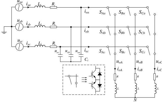
where 𝐮e, 𝐢e, 𝐮o and 𝐢o present the input voltage, the input current, the output voltage and the load current of the DMC, respectively. SXY (X∈ {A, B, C}, Y∈ {a, b, c}) equals to ‘1’ when SXY is turned on and equals to ‘0’ when SXY is turned off, respectively.

uoC uoA uoB

ioB ioA usa usb usc iea R Ci ieb isa isb ioC R R ea u ec

u ueb isc

Li Ri

Li Ri

Li Ri

iec SAa SAb SAc SBa SBb SBc SCa SCb SCc N L L L

Fig. 1 The topology of the direct matrix converter

3.

Principle of predictive control

In the following section all the three phase quantities are assumed to be symmetrical and these can therefore be transformed from the static three-phase coordinates to the static two-phase coordinates. For example, certain three phase quantities Xa, Xb and Xc are re-expressed by the complex space vector

X



X

 

j X

1

(2 )

3 1

( )

3

a b c

b c

X X X X

X X X





 _{  }

 

 _{ }

 (5)

Predictive control is utilized to select the optimal switching state that makes the controlled variables follow the respective reference during one sample period. For DMC, two main conditions must be satisfied to properly operate: unity power factor and satisfactory steady state performance. The predictive values of the source and load currents are calculated for each possible switching state by measuring the source voltage, the source current, the capacitor voltages and the load current to meet the mentioned objectives. First, the objective of unity power factor can be reduced to keep the source voltage and current in the same phase, as follow



 



1

P P

s s s s

g  i i  ii ₍₆₎

where 𝑖𝑠𝛼𝑃 and 𝑖𝑠𝛽𝑃 denote the predictive source current in the next sample period and 𝑖𝑠𝛼∗ and 𝑖𝑠𝛽∗ denote the respective references. The phase of source current reference is equal to the phase of source voltage, and the amplitude of source current reference is determined as follow [11]





* 4

2

sm sm i om

sm

i

U U R RI

I

R









 

 (7)

where 𝐼_𝑜𝑚∗ and 𝑈_𝑠𝑚 are the amplitude of the reference load current and the source voltage, respectively. 𝜂 means the efficiency of DMC.

Second, the objective of satisfactory steady state performance can be reduced to minimize the error between the load current prediction and reference



 



2

P P

o o o o

g  i i  i i ₍₈₎

where 𝑖_𝑜𝛼𝑃 and 𝑖_𝑜𝛽𝑃 denote the predictive load current in the next sample period and 𝑖_𝑜𝛼∗ and 𝑖_𝑜𝛽∗ denote the respective references. Equations (6) and (8) are merged into a cost function

1 1 2 2

g

  



g





g

where λ1, λ2 are the weighing factors deciding the priority of corresponding control variable, which are flexibly changed due to different control requirements. At each sample period, all possible switching states are substituted into (9) to calculate g. The switching state generating the minimum value of g is selected to be implemented for the next sample period.

4.

Calculation of predictive values

mathematical models of input filter and load.

The mathematical model of the input filter is related to the source voltage, input voltage, source current and input current, and the following state-space system describe the input filter model

e e s

s s e

du dt u u

A B

di dt i i

                    (10)

0 1 / 0 1 /

,

1 / / 1 / 0

i i

i i i i

C C

A B

L R L L



   

_{ } _{ }

 

    (11)

where the us, ue, is, ie represent the source voltage, input voltage, source current and input current, respectively. Ri, Li, Cirepresent the resistances, inductances and capacitance of the mains and filter, respectively. Further, assuming the sample period is Ts, the state-space system is discretized by Forward Euler Approximation and the predictions of capacitor voltage and source current are obtained as follow

1

1

1 ( )

s s

k k k

AT AT

e e s

k k k

s s e

u u u

e A e I B

i i i

                 

      (12)

The load model is related to the output voltage and load current, and the following state-space system describes the load model

o

o o

di

L

u

Ri

dt





which is discretized in the same way as follow 1

(1 )

k k k

o o s s o

i  u T L T R L i (14) Above all, all the prediction equations are rewritten as follow

1

11 12 11 12

1

21 22 21 22

1

1 2

k k k k k

e e s s e

k k k k k

s e s s e

k k k

o o o

u

L u

L i

M u

M i

i

L u

L i

M u

M i

i

N u

N i

  













_

_

_

_





_

_



where 11 12 21 22

= ATs

L L e L L       ,

11 12 1

21 22

= ( ATs )

M M

A e I B

M M         , 1 2 1 s s

N T L

N T R L

 

 _{ }

 .

5.

Proposed Predictive Control with Preselection Algorithm

substituted into the cost function for optimum selection when the input current vector and the output voltage vector lie in different sectors respectively.

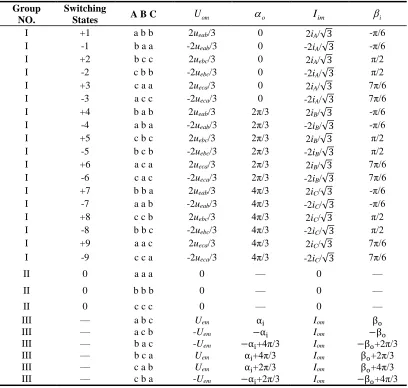
According to the output voltage vector and input current vector that each switching state generates, the 27 switching states are classified into three groups as shown in Table 1, where 𝑢𝑒𝑖𝑙 (i, l





Group I: Two output phases are connected to a common input phase, and the third is connected to a different input phase. This group includes 18 switching states which represent the active vectors and determine the output voltage vector and input current vector.

Group II: All three output phases are connected to the same input phase. This group includes three switching states which determine zero input current and output voltage vectors.

Table. 1 Possible switching states and their space vectors Group

NO.

Switching

States A B C

U



I



I +1 a b b 2ueab/3 0 2iA/√3 -π/6

I -1 b a a -2ueab/3 0 -2iA/√3 -π/6

I +2 b c c 2uebc/3 0 2iA/√3 π/2

I -2 c b b -2uebc/3 0 -2iA/√3 π/2

I +3 c a a 2ueca/3 0 2iA/√3 7π/6

I -3 a c c -2ueca/3 0 -2iA/√3 7π/6

I +4 b a b 2ueab/3 2π/3 2iB/√3 -π/6

I -4 a b a -2ueab/3 2π/3 -2iB/√3 -π/6

I +5 c b c 2uebc/3 2π/3 2iB/√3 π/2

I -5 b c b -2uebc/3 2π/3 -2iB/√3 π/2

I +6 a c a 2ueca/3 2π/3 2iB/√3 7π/6

I -6 c a c -2ueca/3 2π/3 -2iB/√3 7π/6

I +7 b b a 2ueab/3 4π/3 2iC/√3 -π/6

I -7 a a b -2ueab/3 4π/3 -2iC/√3 -π/6

I +8 c c b 2uebc/3 4π/3 2iC/√3 π/2

I -8 b b c -2uebc/3 4π/3 -2iC/√3 π/2

I +9 a a c 2ueca/3 4π/3 2iC/√3 7π/6

I -9 c c a -2ueca/3 4π/3 -2iC/√3 7π/6

II 0 a a a 0 — 0 —

II 0 b b b 0 — 0 —

II 0 c c c 0 — 0 —

III — a b c Uem αi Iom βo

III — a c b -Uem −αi Iom −βo

III — b a c -Uem −αi+4π/3 Iom −βo+2π/3

III — b c a Uem αi+4π/3 Iom βo+2π/3

III — c a b Uem αi+2π/3 Iom βo+4π/3

III — c b a -Uem −αi+2π/3 Iom −βo+4π/3

current vectors have variable directions and amplitudes. Thus, the remaining six switching states are difficult to synthesize the reference vectors.

As shown in Fig. 2, the complex plane is divided into six sectors by six active voltage vectors. At any sample period, the reference output voltage 𝑢𝑜∗ can be calculated from the reference load current 𝑖𝑜∗ and the resistance-inductance load. The reference input current 𝑖𝑒∗ can be obtained from the source voltage 𝑢𝑠 and the reference source current 𝑖𝑠∗. The following equations describe the relationship among the quantities above.

* *

o

( )

o o

u  Rj



*

* *

( )

s e i i i s

s c e

c i i e

u u R j L i

i i i

i j C u





   

 _{ }    

(17)

where R and L are the load resistance and inductance respectively. Li comprises the mains and filter inductances, Ri represents the mains and filter resistances and Ci is the filter capacitance. For the preselection of the finite control set, it is necessary to judge the sector of the vector 𝑢𝑜∗ and 𝑖𝑒∗. Assume the input power factor is unity, the angle of the vector 𝑢𝑜∗ and 𝑖𝑒∗ can be calculated as follows.

o

arctan

o uo i

L

R











*

2 2 *

( )

arctan

(1 )

i i s i s ie is

i i s C u R i

C i









 

 

 (19)

where 𝛼𝑢𝑜 is the angle of the vector 𝑢𝑜∗, 𝛼𝑖𝑜 is the angle of the vector 𝑖𝑜∗. 𝛽𝑖𝑒 is the angle of the vector 𝑖𝑒∗ and 𝛽𝑖𝑠 is the angle of the source 𝑖𝑠∗.

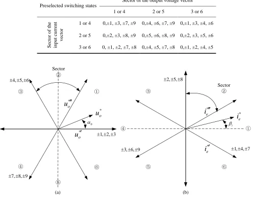
In order to clearly explain the method of preselecting the finite control set, the reference vectors 𝑢_𝑜∗ and 𝑖_𝑒∗ are both assumed to be located in sector I as shown in Fig. 2 (a) and (b). The reference voltage vector 𝑢_𝑜∗ is resolved into two adjacent vectors 𝑢_𝑜∗′ and 𝑢_𝑜∗′′. The vector 𝑢_𝑜∗′ can be synthesized with the voltage vectors which correspond to the pairs of switching configurations ±1, ±2, ±3. These voltage vectors have the same direction with 𝑢𝑜∗′. At the same time, the six switching states of 𝑢𝑜∗′′ are ±7, ±8, ±9. Similarly, the reference input current vector 𝑖𝑒∗ is obtained from two adjacent vectors 𝑖𝑒∗′ and 𝑖𝑒∗′′ which are generated by switching configurations ±3, ±6, ±9 and ±1, ±4, ±7. But only the common switching states between the output voltage and input current vectors will be considered in the finite control set because they are synthesized at the same sample period. As a result, the switching states ±2 and ±8 are eliminated and the switching configurations ±1, ±3, ±7, ±9 will be selected in the finite control set.

Preselected switching states

Sector of the output voltage vector

1 or 4 2 or 5 3 or 6

Secto r o f th e in p u t cu rr en t v ec to r

1 or 4 0,±1, ±3, ±7, ±9 0,±4, ±6, ±7, ±9 0,±1, ±3, ±4, ±6 2 or 5 0,±2, ±3, ±8, ±9 0,±5, ±6, ±8, ±9 0,±2, ±3, ±5, ±6 3 or 6 0, ±1, ±2, ±7, ±8 0,±4, ±5, ±7, ±8 0,±1, ±2, ±4, ±5

① Sector ② ③ ④ ⑤ ⑥

2, 5, 8   

3, 6, 9

     1, 4, 7

* e

i

i



i



4, 5, 6   

7, 8, 9   

1, 2, 3    0  * o

u

u



u



Fig. 2 (a) Ouput voltage vectors generated by the active switching states (b) Input current vectors generated by the active switching states

In the same way, it is possible to determine the eight switching states related to any possible combination of output voltage and input current sectors. On the other hand, the three switching states from group II are chosen in each finite control set because the zero input current and output voltage vectors are useful for the proposed predictive control method. The preselected switching states are summarized in Table 2. In Fig. 3, the block diagram of the predictive control strategy applied on DMC is described. At the kth _{sample period T}k_{, the angles of reference input current vector and the reference output voltage vector are computed from (18)} and (19). With the angle of the vector 𝑖𝑒∗ and 𝑢𝑜∗, it is easy to judge the sectors of 𝑖𝑒∗ and 𝑢𝑜∗. And there are eleven switching states chosen in the preselected finite control set. At the same time, the variables 𝑢_𝑠𝑘, 𝑖_𝑠𝑘, 𝑢_𝑒𝑘 and 𝑖_𝑜𝑘 in Tk _{are obtained from the sensor} circuits, and the switching states Sk _{in T}k _{is obtained from the previous sample period. The variables 𝑖}

sample period. In the same way, predictive values of 𝑖𝑜𝑘+2 and 𝑖𝑠𝑘+2 at the (k+2)th sample period Tk+2 can be obtained for each valid switching state. Substituting each predictive value into gk+2_{, the switching state making g}k+2 _{minimal will be applied in the (k+1)}th sample period Tk+1_.

Switching state selection

gk+2 Input filter

model Load model

Source

DMC

Input filter

model Load model

Preselecting the finite control set refer to Table 2 Judging the sector MC model * o

i

i

i

u

i

u

i

u

R

_R

L

_L

C

i

u

i

i

i

i

2 k s

i

u

Fig. 3 Block diagram of the predictive control strategy

6.

Experimental Results

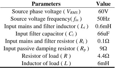
The operation of the DMC using model predictive control with the preselection algorithm has been experimental validated using a prototype converter. Using the full schematic model of the system, all the experiments are performed with a symmetrical three phase source. The setup is fed at 50Hz and the output fundamental frequency was chosen as 40Hz or 60Hz in order to ensure the universality of the experiments. Relevant parameters of the experimental converter are presented in Table 3. The power source isn’t perfect and hence the AC source voltages contain some undesirable fifth-order and seventh-order harmonics. Thus, the value of Rp is chosen as 9Ω, slightly higher than the ideal value. The bi-directional switches are implemented using IGBT modules, FF200R12KT3_E. Sensor circuits are equipped to provide the information of the source voltage, the source current, the capacitor voltage and the load current. A floating-point digital signal processor (DSP, TMS320F28335) is used to select the optimal switching state while a field programmable gate array (FPGA, EP2C8T144C8N) is used for generating a set of impulses to control the switches. The floating-point DSP can also show the computation time of the system.

Table. 3 Parameters of the low-voltage experimental prototype

Parameters Value

Source phase voltage ( VRMS ) 60V Source voltage frequency( fin) 50Hz Input mains and filter inductor ( Li) 0.6mH

Input filter capacitor ( Ci) 66uF Input mains and filter resistor ( Ri ) 0.1Ω Input passive damping resistor ( Rp ) 9Ω

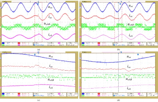
The experiment results comparing the conventional and proposed method are shown in Fig. 4 when the amplitude of the reference load current change. 𝑢_𝑠𝑎, 𝑖_𝑠𝑎, 𝑢_𝑜𝐴𝐵 and 𝑖_𝑜𝐴 represent the source voltage, the source current, the output line-to-line voltage and the load current, respectively. The enlarged drawings of the red dotted box in Fig. 4(a), (c) are shown in Fig. 4(b), (d), respectively. The transient response time of the proposed method in Fig. 4(b), (d) is about 0.4ms, which is similar to the conventional method in Fig. 4(a), (c).

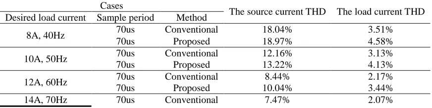
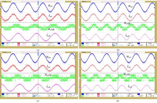
The experiment results of the proposed method with different reference load current are shown in Fig. 5. At the same time, the conventional method is also experimented to make a comparison. Furthermore, experiments are performed to show a good result with the unit power factor and the load current following the reference accurately. Because 27 switching states are considered for the conventional method while only 11 switching states are considered for the preselection algorithm. The computation time of the conventional method for DSP (TMS320F28335) is about 64.1us while the less computation time 33.73us is taken by the preselection algorithm. The detailed comparison between the running time required by the conventional method and the proposed method are shown in Table. 4. Experimental results with the same 𝐼𝑜𝑚∗ /𝑓𝑜 value are performed. The THD values of the source current and the load current with conventional method (Ts=70us) and proposed method (Ts=70us) are described in Table 5. The THD values of the proposed method with Ts=70us are a little larger than those of the conventional method with Ts=70us.

The experimental waveforms of the preselection algorithm show almost the same performance as that of the conventional method. Because of the time the preselection algorithm saves, it is possible to implement the total algorithm on microcontroller, which is cheaper and has lower calculating speed. In other words, these time savings allow the microcontroller to implement some other operations in only one sample period. Certainly, if high performance is required and the cost of microcontroller is negligible, the conventional method should be considered.

Table. 4 Comparison between the running time required by the conventional method and the proposed method Case

(Ts =70us)

Time (us)

A/D conversion FCS-MPC algorithm Other algorithms Free

Conventional method 2.63 55.25 4.42 5.90

Proposed method 2.63 26.50 4.60 36.27

Table. 5 THD values of the source current and the load current Cases

The source current THD The load current THD Desired load current Sample period Method

8A, 40Hz 70us Conventional 18.04% 3.51%

70us Proposed 18.97% 4.58%

10A, 50Hz 70us Conventional 12.16% 3.13%

70us Proposed 13.22% 4.13%

12A, 60Hz 70us Conventional 8.44% 2.17%

70us Proposed 10.04% 3.44%

70us Proposed 9.35% 3.17%

(d) (c)

u

i

u

i

(b) (a)

u

i

u

i

u

i

u

i

u

i

u

i

Fig. 4 Experiment results with Ts =70us when the reference load current changes from 𝐼𝑜𝑚∗ = 8A, fo = 40Hz to 𝐼𝑜𝑚∗ = 12A, fo = 40Hz (a) Conventional method. (b) Proposed method. (c) The enlarged drawing of the red dotted box in (a). (d) The enlarged

(c) (d)

u

i

u

i

(a) (b)

u

i

u

i

u

i

u

i

u

i

u

i

Fig. 5 Experiment results with Ts =70us. Conventional method: (a) 𝐼𝑜𝑚∗ = 8A, fo = 40Hz. (b) 𝐼𝑜𝑚∗ = 12A, fo = 60Hz. Proposed method: (c) 𝐼𝑜𝑚∗ = 8A, fo = 40Hz. (d) 𝐼𝑜𝑚∗ = 12A, fo = 60Hz.

7.

Conclusion

In this paper a predictive control method with a preselection algorithm for a Matrix Converter is proposed. On the premise of satisfying the conditions of unity input power factor and accurately following the output current reference value, the proposed control method can reduce the calculation effort for the model predictive controller. The proposed method could also be used with a shorter sample period because of lower computation time. The proposed method preselects the finite control set by judging the sectors of the input current vector and the output voltage vector; only the switching states in the preselected finite control set are considered while the conventional predictive control method enumerates all the switching states satisfying the restriction of the matrix converter topology. The proposed method allows the regulation of the input power factor by controlling the phase shift between the source current and the source voltage. The experiment results validate the feasibility of the method.

8.

References

[1] Kazmierkowski, M.P., Krishnan, R., Blaabjerg, F.: ‘Control in power electronics’, New York, 2002.

[3] Cortés, P., Kazmierkowski, M. P., Kennel, R. M., et al.: ‘Predictive control in power electronics and drives’, IEEE Trans. Ind. Electron., 2008, 55, (12), pp.

4312-4324.

[4] Kouro, S., Cortes, P., Vargas, R., Ammann, U., and J. Rodriguez.: ‘Model predictive control, a simple and powerful method to control power converters’,

IEEE Trans. Ind. Electron., 2009, 56, (6), pp. 1826-1838.

[5] Kouro, S., Perez, M. A., Rodriguez, J., Llor, A. M., Young, H. A.:‘Model predictive control: mpc's role in the evolution of power electronics’,IEEE Trans.

Ind. Electron., 2014, 9, (4), pp. 8-21.

[6] Rivera, M., Rojas, C., Rodriguez, J., Espinoza, J.: ‘Methods of source current reference generation for predictive control in a direct matrix converter’, IET

Power Electron., 2013, 6, (5), pp. 894–901.

[7] Rivera, M., Rojas, C., Wilson, A. et al.: ‘Review of predictive control methods to improve the input current of an indirect matrix converter’, IET Power

Electron., 2014, 7, (4), pp. 886–894.

[8] Uddin, M., Mekhilef, S., Rivera, M.:‘Experimental validation of minimum cost function-based model predictive converter control with efficient reference

tracking’, IET Power Electron., 2015, 8, (2), pp. 278–287.

[9] Uddin, M., Mekhilef, S., Rivera, M.et al.:‘Imposed weighting factor optimization method for torque ripple reduction of im fed by indirect matrix converter

with predictive control algorithm” Journal of Electrical Engineering and Technology, 2015, 10, (1), pp. 227–242.

[10] Jasinski, M., Kazmierkowski, M., Malinowski, M.:‘Model predictive control for 3-level 4-leg flying capacitor converter operating as shunt active power

filter'. Proc. Int. Conf. Industrial Technology, Seville, Spain, March 2015.

[11] Peng T., Dan H., Yang J. et al.: ‘Open-switch fault diagnosis and fault tolerant for matrix converter with finite control set-model predictive control’, IEEE

Trans. Ind. Electron., 2016, 63, (9), pp. 5953-5863.

[12] Wheeler, P.W., Rodríguez, J., Clare, J.C., Empringham, L., Weinstein, A.: ‘Matrix converters: a technology review’, IEEE Trans. Ind. Electron., 2002, 49, (2),

pp. 276-288.

[13] Gyugyi, L.: ‘Generalized theory of static power frequency changers’, PhD thesis, University of Salford, 1970.

[14] Koiwa, K., Itoh, J.I.:‘A maximum power density design method for nine switches matrix converter using sic-mosfet’, IEEE Trans. Power Electron., 2016, 31,

(2), pp. 1189-1202.

[15] Abebe, R., Vakil, G., Giovanni L.C.:‘Integrated motor drives: state of the art and future trends’, IET Electric Power Application, 2016, 10, (8), pp. 757-771.

[16] Monteiro, J., Silva, J. F., Pinto, S. F., Palma, J.:‘Matrix converter-based unified power-flow controllers: Advanced direct power control method’, IEEE Trans.

Power Delivery, 2011, 26, (1), pp. 420-430.

[17] Suman, M., Debaprasad, K.:‘Improved direct torque and reactive power controlof a matrix converter fed grid connected doubly fed induction generator’,

IEEE Trans. Ind. Electron., 2015, 62, (12), pp. 7590-7595.

[18] Rodriguez, J., Rivera, M., Kolar, J. W., Wheeler, P. W.: ‘A review of control and modulation methods for matrix converters’, IEEE Trans. Ind. Electron., 2012,

59, (1), pp. 58-70.

[19] Rivera, M., Wheeler, P. W., Olloqui, A.:‘Predictive control in matrix converters - Part I: Principles, topologies and applications'. Proc. Int. Conf. Industrial

Technology, Taipei, Taiwan, March 2016.

[20] Rivera, M., Wheeler, P. W., Olloqui, A.:‘Predictive control in matrix converters - Part II: Control strategies, weaknesses and trends'. Proc. Int. Conf.

Industrial Technology, Taipei, Taiwan, March 2016.

[21] Muller, S., Ammann, U., Rees, S.: ‘New time-discrete modulation scheme for matrix converters’, IEEE Trans. Ind. Electron., 2005, 52, (6), pp. 1607-1615.

[22] Linder, A., Kanchan, R., Kennel, R., Stolze, P.: ‘Model-based predictive control of electric drives’, Cuvillier Verlag, 2010.

[23] Stolze, P., Landsmann, P., Kennel, R., Mouton, T.: ‘Finite-set model predictive control with heuristic voltage vector preselection for higher prediction

[24] Stolze, P., Tomlinson, M., Kennel, R., Mouton, T.: ‘Heuristic finite-set model predictive current control for induction machines'. Proc. Int. Conf. ECCE Asia

Downunder, Melbourne, Australia, June 2013, pp. 1221-1226.

[25] Cortés, P., Wilson, A., Kouro, S., Rodriguez, J., Abu-Rub, H.: ‘Model predictive control of multilevel cascaded h-bridge inverters’, IEEE Trans. Ind.

Electron., 2010, 57, (8), pp. 2691-2699.

[26] Tarisciotti, L., Calzo, G.L., Gaeta, A., Zanchetta, P., Valencia, F., Saez, D.:‘A distributed model predictive control strategy for back-to-back converters’,

IEEE Trans. Ind. Electron., 2016, 63, (9), pp. 5869-5878.

[27] Xia, C., Liu, T., Shi, T., Song, Z.:‘A simplified finite-control-set model-predictive control for power converters’, IEEE Trans. Ind. Informatics, 2014, 10, (2),