Sensorless speed control of five phase PMSM drives with low current distortion

(1)

Sensorless Speed Control of Five-Phase PMSM Drives with Low

Current Distortion

Abstract

This paper introduces a design for a sensorless control of a five-phase PMSM drive working at low and zero speeds with low current distortion. The rotor position is obtained through tracking the saturation saliency by measuring the dynamic currents responses of the motor due to the IGBTs switching actions. It uses the fundamental PWM waveform obtained using the multi-phase space vector pulse width modulation only. The saliency tracking algorithm used in this paper doesn’t only improve the quality of the estimated position signals but also guarantees a minimum current distortion through reducing the modifications introduced on the PWM waveform. Simulation results are provided to verify the effectiveness of the proposed strategy for saliency tracking and current distortion minimizing of a five-phase PMSM motor drive over a wide speed ranges under different load conditions.

Keywords: Sensorless, five-phase motor, multi-dimension SVPWM, THD.

1. Introduction

The interest in multi-phase motor drives has increased in recent years as they offer several advantages when compared to three-phase machines such as improving reliability, efficiency and torque density and reducing torque pulsations [1, 2] . Therefore, multi-phase motor drives are extensively considered for applications related to vehicles, aerospace application (more electric craft), ship propulsion and high power applications. The modulation technique that is proposed for using in multi-phase motor drives is multi-dimension SVPWM which is based on the concept of orthogonal multi-dimensional vector space [3, 4, 5, 6, 7, 8, 9, 10, 11, 12]. This modulation technique can synthesize voltage vectors both in d-q subspace and in other subspace. Many control techniques has been adopted to control the multi-phase motor drives in sensored mode such as fuzzy logic control [13], predictive current control [14].

In the last couple of years, few researches have been directed towards the sensorless control of a multi-phase electrical drives. These researches focus on the model based sensorless control, direct torque control and high frequency injections[15, 16, 17, 18, 19].

This paper introduces a new method to track the saturation saliency in five-phase PMSM drives to obtain the rotor position through measuring the dynamic currents responses of the motor due to the IGBTs switching actions [20,21,22]. It uses the fundamental PWM waveform obtained using the multi-phase space vector pulse width modulation only. The saliency tracking algorithm used in the proposed method doesn’t only improve the quality of the estimated position signals but also guarantees a minimum current distortion in the motor currents through reducing the modifications introduced on the PWM waveform.

2. Research Method

2.1 Five-phase converter drive topology

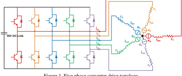
Figure 1 shows the proposed phase converter drive topology [17]. The model of the motor is a five-phase model not a d-q model to make the results more realistic. Also the saturation saliency (2*fe) is embedded in the motor equations.

INV DC Link

ia

lσa

ea rs

lσd ed

rs _l

σe

ee

rs lσb

eb

rs

lσc

ec

rs

[image:1.595.138.455.583.715.2]

ib ic id ie

Figure 1. Five phase converter drive topology.

(2)

The kth order harmonics (k = 5×m ± 2, m = 1,3,5...) of the machine's variables such as phase voltage, phase current which do not produce any rotating MMF and are non electromechanical energy conversion related will freely flow through the windings of the five-phase motors and their amplitude will be restricted by the stator leakage impedance only [3-12 , 15-19]. Hence, generation of certain low-order voltage harmonics (3rd harmonic) in the VSI output can lead to large 3rd harmonic in stator current. It is therefore important that the multi-phase VSI output is kept as close as possible to sinusoidal. To do so, the reference voltage should be mapped into two orthogonal planes. The first one is the d1-q1 plane that is rotating at synchronous speed and has fundamental components of the reference voltage. The second is the d3-q3 plane that is rotating at 3 times the synchronous speed and has the 3rd harmonic components of the reference voltage using the transformation given in (1) and (2):-

[ 𝑑1 𝑞1 𝑑3 𝑞3

] = [𝐺]

[ 𝑎 𝑏 𝑐 𝑑 𝑒]

.. (1) and

= [𝐺−1_{] [}

𝑑1 𝑞1 𝑑3 𝑞3

].. (2) Where

G= 2₅

[

sin(𝜃) sin (𝜃 − 72°) sin (𝜃 − 144°) sin (𝜃 − 216°) sin (𝜃 − 288°) cos(𝜃) cos (𝜃 − 72°_{) cos (𝜃 − 144}°_{) cos (𝜃 − 216}°_{) cos (𝜃 − 288}°₎

sin (3𝜃) sin (3(𝜃 − 72°_{)) sin (3(𝜃 − 144}°_{)) sin (3(𝜃 − 216}°_{)) sin (3(𝜃 − 288}°₎₎

cos (3𝜃) cos(3(𝜃 − 72°_{)) cos (3(𝜃 − 144}°_{)) cos(3(𝜃 − 216}°_{)) cos (3(𝜃 − 288}°_))]

(3)

As the two planes d1-q1 and d3-q3 are orthogonal, the fundamental and the third harmonic components of the voltage can be controlled independently. Also the reference voltage can be mapped into two orthogonal stationary frames α1-β1 and α3-β3 according to (4,5,6).

[ 𝛼1 𝛽1 𝛼3 𝛽3

] = [𝐻]

…….. (4) And

= [𝐻−1_{] [}

𝛼1 𝛽1 𝛼3 𝛽3

]…. (5) , Where

𝐻 = 2₅

[

1 cos(72°) cos(144°) cos (216°) cos (288°) 0 sin (72°_{) sin(144}°_{) sin (216}°_{) sin (288}°₎

1 cos(216°_{) cos(72}°_{) cos (288}°_{) cos (144}°₎

0 sin(216°_{) sin(72}°_{) sin (288}°_{) sin (144}°_)]

……….. (6)

Using the equation (4, 5, 6) there are 32 space vectors, two of which are zero vectors(00000 and 11111). Thirty non-zero space voltage vectors of a five-phase inverter can be projected to α1-β1 plane and α3-β3 palne as shown in Figure 2. In α1-β1 palne, the thirty vectors are composed of three sets of different amplitude vectors, and divide α1-β1 plane into 10 sectors. The amplitudes of these voltage vectors are [3-12, 15]:-

Vmin = 0.2472Vdc, (11001), (11000), (11100), (01100), (01110), (00110), (00111), (00011), (10011), (10001).

Vmid = 0.4Vdc, (10000), (11101), (01000), (11110), (00100),(01111), (00010), (10111), (00001), (11011). Vmax = 0.6472Vdc, (01001), (11010), (10100), (01101), (01010), (10110), (00101), (01011), (10010), (10101). And the ratio of the amplitudes is 1:1.618:1.6182. It is the same situation in the α3-β3 plane.

sector2

sector1 sector3

sector4

sector5

sector6

sector7

sector8 sector9

sector10

(00011) (01000)

(01001)

(11100) (10111)

(10100)

(01101)

(01010)

(11000) (01001)

(10001)

(00101)

(11101)

(00111)

(01010)

(00100)

(11001) (01111)

(11010) (00010) (01110)

(11011)

(01100) (00001)

(11110) (10011)

(10000)

(00110) α 3

β 3

Phase a

Phase b

Phase c

Phase d Phase e

sector2

sector1 sector3

sector4

sector5

sector6

sector7

sector8 sector9

sector10

(11100)

(01000)

(10100)

(11010) (11101)

(11000)

(11001)

(10001)

(10011)

(00011) (00111)

(00110)

(01110)

(01100)

(11110)

(01101)

(01010) (00100)

(10110) (01111)

(00101)

(00010) (01011)

(10111)

(10010)

(00001)

(11011) (10101)

(10000)

(01001) α1

β 1

Phase a

Phase b

Phase c

Phase d

Phase e

[image:2.595.128.474.551.721.2]

(10110)

Figure 2. Thirty nonzero switching vectors on α1 –β1 plane and α3 –β3 plane.

(3)

Vmax switching vectors. The other combinations of switching vectors increase the number of switching or decrease the maximum magnitude of the realizable voltage vector.

2.2.2 Calculation of the Application Times for the Switching Vectors

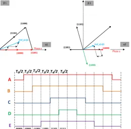
Figure 3 shows the reference voltage of the fundamental component ( Vref_ α1-β1) exists in the first quadrant in the α1-β1 plane and the third harmonic component of the reference voltage (Vref_ α3-β3) located in the first sector in the α3-β3 plan. For both reference voltages, the vectors (00000, 10000, 11000, 01001, 11101, 11111) are used to utilize them in both α1-β1 and α3-β3 planes as shown in figure 3.

(11101) (11000)

(11001) (10000)

α1 β 1

Phase a

(11000) (11101)

(11001) (10000)

α3 β 3

Phase a Vref_α1-β1

Vref_α3-β3

A

B

C

D

E

T0/2 T1/2 T2/2 T3/2 T4/2 T0/2

[image:3.595.172.432.183.439.2]

00000 10000 11000 11001 11101 11111

Figure 3. Realization of a reference voltage vector located in sector 1 on the d –q plane and the associated switching sequence

The time needed for applying each vectors can be calculated as:-

[ 𝑇1 𝑇2 𝑇3 𝑇4

] = 𝑇𝑠 × [𝑇−1_{] [}

Vref_ α1 Vref_ 𝛽1 Vref_ 𝛼3 Vref_ 𝛽3

] ….. (7) Where

T =

[

𝑉𝑚𝑖𝑑 𝑉𝑚𝑎𝑥cos(72°) 𝑉𝑚𝑎𝑥 𝑉𝑚𝑖𝑑cos(72°) 0 𝑉𝑚𝑎𝑥sin (72°) 0 𝑉𝑚𝑖𝑑sin (72°)

𝑉𝑚𝑖𝑑 𝑉𝑚𝑖𝑛cos(288°) −𝑉𝑚𝑖𝑛 𝑉𝑚𝑖𝑑cos(108°)

0 𝑉𝑚𝑖𝑛sin (288°) 0 𝑉𝑚𝑖𝑑sin (108°)]

……….. (8)

𝑇0= 𝑇𝑠− 𝑇1− 𝑇2− 𝑇3− 𝑇4 ……….. (9)

The same approach can be applied for other sectors.

2.3 Algorithm for tracking the saturation saliency of five phase PMSM

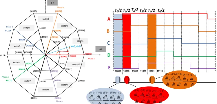
The stator windings self-inductances are modulated by the anisotropy obtained by the saturation saliency of main flux as shown in [20]. This modulation will be reflected in the transient response of the motor line currents to the test vector imposed by the inverter. So by using the fundamental PWM wave form and by measuring the transient current response to the active vectors, it is possible to detect the inductance variation and track the rotor position. It is worth to say here that the output PWM waveform obtained using the multi-dimension SVPWM in this work has four active vectors V1,V2,V3,and V4 in addition to the zero vector V0. This number of active vectors make it possible to obtain more than one algorithm to track the saturation saliency. This paper introduces the following algorithms:

2.3.1 Tracking saliency using the active vectors V1,V4 and V0

(4)

A

B

C

D

E

T0/2 T1/2 T2/2 T3/2 T4/2 T0/2

00000 10000 11000 11001 11101 11111

[image:4.595.113.488.88.268.2]

dt di V b ) 1 ( dt di V c ) 1 ( dt di V a ) 1 ( dt di V d ) 1 ( dt di V e ) 1 ( dt di V b ) 0 ( dt di V c ) 0 ( dt di V a ) 0 ( dt di V d ) 0 ( dt di V e ) 0 ( dt di V b ) 4 ( dt di V c ) 4 ( dt di V a ) 4 ( dt di V d ) 4 ( dt di V e ) 4 ( sector2 sector1 sector3 sector4 sector5 sector6 sector7 sector8 sector9 sector10 (11100) (01000) (10100) (11010) (11101) (11000) (11001) (10001) (10011) (00011) (00111) (00110) (01110) (01100) (11110) (01101) (01010) (00100) (10110) (01111) (00101) (00010) (01011) (10111) (10010) (00001) (11011) (10101) (10000) (01001) α1 β 1 Phase a Phase b Phase c Phase d Phase e Vref_α1-β1

Figure 4. Sampling time of the currents responses due to the switching actions of active vector V1 and V4 in case that V_ref_α1-β1 exists in first sector

The stator circuit when the vectors V0,V1 and V4 are applied are shown in Figure 5.a, figure 5.b and figure 5.c respectively.

lσa

ea rs

lσd

ed

rs _l

σe ee rs lσb eb rs lσc ec rs VDC+ lσa ea rs lσd ed

rs _l

σe ee rs lσb eb rs lσc ec rs lσa ea rs lσd ed

rs _l

[image:4.595.122.464.324.446.2]

σe ee rs lσb eb rs lσc ec rs VDC + -ia ib ic id ie ia ib ic id ie ia ib ic id ie

Figure 5. Stator circuits when: (a) V0 is applied; (b) V1 is applied; (c) V4 is applied

Using the circuit in Figure 5.a, the following equations hold true:-

0 = 𝑟𝑠∗ 𝑖𝑎(𝑉0)+ 𝑙𝜎𝑎∗𝑑𝑖𝑎 (𝑉0)

𝑑𝑡 + 𝑒𝑎

(𝑉0)_{− 𝑟}

𝑠∗ 𝑖𝑏(𝑉0)− 𝑙𝜎𝑏∗ 𝑑𝑖_𝑏(𝑉0)

𝑑𝑡 − 𝑒𝑏

(𝑉0)_{………. (10)}

0 = 𝑟𝑠∗ 𝑖𝑏(𝑉0)+ 𝑙𝜎𝑏∗

𝑑𝑖_𝑏(𝑉0)

𝑑𝑡 + 𝑒𝑏

(𝑉0)_{− 𝑟}

𝑠∗ 𝑖𝑐(𝑉0)− 𝑙𝜎𝑐∗𝑑𝑖𝑐 (𝑉0)

𝑑𝑡 − 𝑒𝑐

(𝑉0)_{……….. (11)} 0 = 𝑟𝑠∗ 𝑖𝑐(𝑉0)+ 𝑙𝜎𝑐∗𝑑𝑖𝑐

(𝑉0)

𝑑𝑡 + 𝑒𝑐

(𝑉0)_{− 𝑟}

𝑠∗ 𝑖𝑑(𝑉0)− 𝑙𝜎𝑑∗ 𝑑𝑖_𝑑(𝑉0)

𝑑𝑡 − 𝑒𝑑

(𝑉0)_{……….. (12)}

0 = 𝑟𝑠∗ 𝑖𝑑(𝑉0)+ 𝑙𝜎𝑑∗

𝑑𝑖_𝑑(𝑉0)

𝑑𝑡 + 𝑒𝑑

(𝑉0)_{− 𝑟}

𝑠∗ 𝑖𝑒(𝑉0)− 𝑙𝜎𝑒∗𝑑𝑖𝑒 (𝑉0)

𝑑𝑡 − 𝑒𝑒

(𝑉0)_{……….. (13)} 0 = 𝑟𝑠∗ 𝑖𝑒(𝑉0)+ 𝑙𝜎𝑒∗𝑑𝑖𝑒

(𝑉0)

𝑑𝑡 + 𝑒𝑒

(𝑉0)_{− 𝑟}

𝑠∗ 𝑖𝑎(𝑉0)− 𝑙𝜎𝑎∗𝑑𝑖𝑎 (𝑉0)

𝑑𝑡 − 𝑒𝑎

(𝑉0)_{……….. (14)}

The following equations are obtained using Figure 5.b:-

V𝐷𝐶= 𝑟𝑠∗ 𝑖𝑎(𝑉1)+ 𝑙𝜎𝑎∗𝑑𝑖𝑎 (𝑉1)

𝑑𝑡 + 𝑒𝑎

(𝑉1)_{− 𝑟}

(𝑉1)_..₍₁₅₎

𝑑𝑡 + 𝑒𝑏

(𝑉1)_{− 𝑟}

(𝑉1)_{……. (16)} 0 = 𝑟𝑠∗ 𝑖𝑐(𝑉1)+ 𝑙𝜎𝑐∗𝑑𝑖𝑐

(𝑉1)

𝑑𝑡 + 𝑒𝑐

(𝑉1)_{− 𝑟}

(𝑉1)_{…….. (17)}

𝑑𝑡 + 𝑒𝑑

(𝑉1)_{− 𝑟}

𝑠∗ 𝑖𝑒(𝑉1)+ 𝑙𝜎𝑒∗𝑑𝑖𝑒 (𝑉1)

(𝑉1)_{……….. (18)}

−V𝐷𝐶 = 𝑟𝑠∗ 𝑖𝑒(𝑉1)+ 𝑙𝜎𝑒∗𝑑𝑖𝑒

(𝑉1)

𝑑𝑡 + 𝑒𝑒

(𝑉1)_{− 𝑟}

(𝑉1)_{… (19)}

Finally when V4 is applied as shown in Figure 5.c, the following equations hold true:-

𝑑𝑡 + 𝑒𝑎

(𝑉4)_{− 𝑟}

(𝑉4)

……..(20)

𝑑𝑡 + 𝑒𝑏

(𝑉4)_{− 𝑟}

(5)

V𝐷𝐶= 𝑟𝑠∗ 𝑖𝑐(𝑉4)+ 𝑙𝜎𝑐∗𝑑𝑖𝑐 (𝑉4)

𝑑𝑡 + 𝑒𝑐

(𝑉4)_{− 𝑟}

(𝑉4)_……(22)

−V𝐷𝐶 = 𝑟𝑠∗ 𝑖𝑑(𝑉4)+ 𝑙𝜎𝑑∗

𝑑𝑡 + 𝑒𝑑

(𝑉4)_{− 𝑟}

(𝑉4)_…(23) 0 = 𝑟𝑠∗ 𝑖𝑒(𝑉4)+ 𝑙𝜎𝑒∗𝑑𝑖𝑒

(𝑉4)

𝑑𝑡 + 𝑒𝑒

(𝑉4)_{− 𝑟}

(𝑉4)_{……….. (24)}

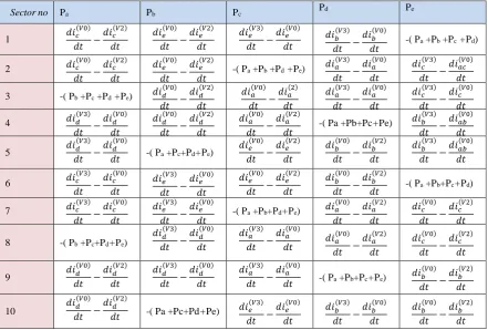
Assuming that the voltage drop across the stator resistances are small and the back emf can be cancelled if the time separation between the vectors is small, the position scalars Pa,Pb,Pc,Pd and Pe in all sectors are given in table 1.

Table1 Selection of Pa, Pb, Pc, Pd and Pe for a star-connected five machine by sampling switching actions of active vector V1 and V4

Sector no Pa Pb Pc Pd Pe

1 𝑑𝑖𝑐

(𝑉0)

𝑑𝑡 −

𝑑𝑖𝑐(𝑉4)

𝑑𝑡

𝑑𝑖𝑒(𝑉0)

𝑑𝑡 −

𝑑𝑖𝑒(𝑉4)

𝑑𝑡

𝑑𝑖𝑒(𝑉1)

𝑑𝑡 −

𝑑𝑖𝑒(𝑉0)

𝑑𝑡 𝑑𝑖𝑏

(𝑉1)

𝑑𝑡 −

𝑑𝑖𝑏(𝑉0)

𝑑𝑡 -( Pa +Pb +Pc +Pd)

2 𝑑𝑖𝑐(𝑉0)

𝑑𝑡 −

𝑑𝑖𝑐(𝑉4)

𝑑𝑡

𝑑𝑖𝑒(𝑉0)

𝑑𝑡 −

𝑑𝑖𝑒(𝑉4)

𝑑𝑡 -( Pa +Pb +Pd +Pe)

𝑑𝑖𝑎(𝑉1)

𝑑𝑡 −

𝑑𝑖𝑎(𝑉0)

𝑑𝑡

𝑑𝑖𝑐(𝑉1)

𝑑𝑡 −

𝑑𝑖𝑎𝑐(𝑉0)

𝑑𝑡

3 -( Pb +Pc +Pd +Pe) 𝑑𝑖𝑑 (𝑉0)

𝑑𝑡 −

𝑑𝑖𝑑(𝑉4)

𝑑𝑡

𝑑𝑖𝑎(𝑉0)

𝑑𝑡 −

𝑑𝑖𝑎(𝑉4)

𝑑𝑡

𝑑𝑖𝑎(𝑉1)

𝑑𝑡 −

𝑑𝑖𝑎(𝑉0)

𝑑𝑡

𝑑𝑖𝑐(𝑉1)

𝑑𝑡 −

𝑑𝑖𝑐(𝑉0)

𝑑𝑡

4 𝑑𝑖𝑑(𝑉1)

𝑑𝑡 −

𝑑𝑖_𝑑(𝑉0) 𝑑𝑡

𝑑𝑡 −

𝑑𝑖𝑎(𝑉0)

𝑑𝑡 −

𝑑𝑖𝑎(𝑉4)

𝑑𝑡 -( Pa +Pb+Pc+Pe)

𝑑𝑡 −

𝑑𝑖_𝑎𝑏(𝑉0) 𝑑𝑡

5 𝑑𝑖𝑑

(𝑉1)

𝑑𝑡 −

𝑑𝑡 -( Pa +Pc+Pd+Pe)

𝑑𝑖𝑒(𝑉0)

𝑑𝑡 −

𝑑𝑖𝑒(𝑉4)

𝑑𝑡

𝑑𝑡 −

𝑑𝑖_𝑏(𝑉4) 𝑑𝑡

𝑑𝑡 −

6 𝑑𝑖𝑐

(𝑉1)

𝑑𝑡 −

𝑑𝑖𝑐(𝑉0)

𝑑𝑡

𝑑𝑖𝑒(𝑉1)

𝑑𝑡 −

𝑑𝑖𝑒(𝑉0)

𝑑𝑡

𝑑𝑖𝑒(𝑉0)

𝑑𝑡 −

𝑑𝑖𝑒(𝑉4)

𝑑𝑡

𝑑𝑡 −

𝑑𝑡 -( Pa +Pb+Pc+Pd)

7 𝑑𝑖𝑐

(𝑉1)

𝑑𝑡 −

𝑑𝑖𝑐(𝑉0)

𝑑𝑡

𝑑𝑖𝑒(𝑉1)

𝑑𝑡 −

𝑑𝑖𝑒(𝑉0)

𝑑𝑡 -( Pa +Pb+Pd+Pe)

𝑑𝑖𝑎(𝑉0)

𝑑𝑡 −

𝑑𝑖𝑎(𝑉4)

𝑑𝑡

𝑑𝑖𝑐(𝑉0)

𝑑𝑡 −

𝑑𝑖𝑐(𝑉4)

𝑑𝑡

8 -( Pb +Pc+Pd+Pe)

𝑑𝑡 −

𝑑𝑖𝑎(𝑉1)

𝑑𝑡 −

𝑑𝑖𝑎(𝑉0)

𝑑𝑡 𝑑𝑖𝑎

(𝑉0)

𝑑𝑡 −

𝑑𝑖𝑎(𝑉4)

𝑑𝑡

𝑑𝑖𝑐(𝑉0)

𝑑𝑡 −

𝑑𝑖𝑐(𝑉4)

𝑑𝑡

9 𝑑𝑖𝑑

(𝑉0)

𝑑𝑡 −

𝑑𝑖𝑎(𝑉1)

𝑑𝑡 −

𝑑𝑖𝑎(𝑉0)

𝑑𝑡 -( Pa +Pb+Pc+Pe) 𝑑𝑖𝑏

(𝑉0)

𝑑𝑡 −

10 𝑑𝑖𝑑

(𝑉0)

𝑑𝑡 −

𝑑𝑡 -( Pa +Pc+Pd+Pe) 𝑑𝑖𝑒

(𝑉1)

𝑑𝑡 −

𝑑𝑖𝑒(𝑉0)

𝑑𝑡

𝑑𝑡 −

2.3.2 Tracking saliency using the vectors V2,V3 and V0

Figure 6 shows the space vector modulation state diagram for a five-phase inverter when V_ref_α1-β1 exists in first sector. The switching sequences and the timing of the applied vectors will be :-

A

B

C

D

E

T0/2 T1/2 T2/2 T3/2 T4/2 T0/2

00000 10000 11000 11001 11101 11111

dt di V b ) 3 ( dt di V c ) 3 ( dt di V a ) 3 ( dt di V d ) 3 ( dt di V e ) 3 ( dt di V b ) 0 ( dt di V c ) 0 ( dt di V a ) 0 ( dt di V d ) 0 ( dt di V e ) 0 ( dt di V b ) 2 ( dt di V c ) 2 ( dt di V a ) 2 ( dt di V d ) 2 ( dt di V e ) 2 ( sector2 sector1 sector3 sector4 sector5 sector6 sector7 sector8 sector9 sector10 (11100) (01000) (10100) (11010) (11101) (11000) (11001) (10001) (10011) (00011) (00111) (00110) (01110) (01100) (11110) (01101) (01010) (00100) (10110) (01111) (00101) (00010) (01011) (10111) (10010) (00001) (11011) (10101) (10000) (01001) α1 β 1 Phase a Phase b Phase c Phase d Phase e Vref_α1-β1

[image:5.595.73.526.202.504.2]

(6)

The stator circuit when the vectors V0,V2 and V3 are applied are shown in Figure 7.a, figure 7.b and figure 7.c respectively.

lσa

ea rs

lσded

rs ee_lσe

rs lσb eb rs lσc ec rs VD C + lσa

ea rs

lσded

rs ee_lσe

rs lσb eb rs lσc ec rs lσa

ea rs

lσded

rs ee_lσe

rs lσb eb rs lσc ec rs VD C + -ia ib ic id ie ia ib ic id ie ia ib ic id ie

-Figure 7. Stator circuits when: (a) V0 is applied; (b) V2 is applied; (c) V3 is applied

Using the circuit in Figure 7.a, the following equations hold true:-

𝑑𝑡 + 𝑒𝑎

(𝑉0)_{− 𝑟}

(𝑉0)_{………. (25)}

𝑑𝑡 + 𝑒𝑏

(𝑉0)_{− 𝑟}

(𝑉0)_{……….. (26)} 0 = 𝑟𝑠∗ 𝑖𝑐(𝑉0)+ 𝑙𝜎𝑐∗𝑑𝑖𝑐

(𝑉0)

𝑑𝑡 + 𝑒𝑐

(𝑉0)_{− 𝑟}

(𝑉0)_{……….. (27)}

𝑑𝑡 + 𝑒𝑑

(𝑉0)_{− 𝑟}

(𝑉0)_{……….. (28)} 0 = 𝑟𝑠∗ 𝑖𝑒(𝑉0)+ 𝑙𝜎𝑒∗𝑑𝑖𝑒

(𝑉0)

𝑑𝑡 + 𝑒𝑒

(𝑉0)_{− 𝑟}

(𝑉0)_{……….. (29)}

The following equations are obtained using Figure 7.b:-

𝑑𝑡 + 𝑒𝑎

(𝑉1)_{− 𝑟}

(𝑉2)_..

(30)

V𝐷𝐶= 𝑟𝑠∗ 𝑖𝑏(𝑉2)+ 𝑙𝜎𝑏∗

𝑑𝑡 + 𝑒𝑏

(𝑉2)_{− 𝑟}

(𝑉2)_{……. (31)} 0 = 𝑟𝑠∗ 𝑖𝑐(𝑉2)+ 𝑙𝜎𝑐∗𝑑𝑖𝑐

(𝑉2)

𝑑𝑡 + 𝑒𝑐

(𝑉2)_{− 𝑟}

(𝑉2)_{…….. (32)}

𝑑𝑡 + 𝑒𝑑

(𝑉2)_{− 𝑟}

𝑠∗ 𝑖𝑒(𝑉2)+ 𝑙𝜎𝑒∗𝑑𝑖𝑒 (𝑉2)

(𝑉2)_{……….. (33)}

−V𝐷𝐶 = 𝑟𝑠∗ 𝑖𝑒(𝑉2)+ 𝑙𝜎𝑒∗𝑑𝑖𝑒

(𝑉2)

𝑑𝑡 + 𝑒𝑒

(𝑉2)_{− 𝑟}

(𝑉2)_{… (34)}

Finally when V3 is applied as shown in Figure 7.c, the following equations hold true:-

𝑑𝑡 + 𝑒𝑎

(𝑉3)_{− 𝑟}

(𝑉3)

……..(35)

V𝐷𝐶= 𝑟𝑠∗ 𝑖𝑏(𝑉3)+ 𝑙𝜎𝑏∗

𝑑𝑡 + 𝑒𝑏

(𝑉3)_{− 𝑟}

(𝑉3)_{……….. (36)}

0= 𝑟𝑠∗ 𝑖𝑐(𝑉3)+ 𝑙𝜎𝑐∗𝑑𝑖𝑐 (𝑉3)

𝑑𝑡 + 𝑒𝑐

(𝑉3)_{− 𝑟}

(𝑉3)_……(37)

−V𝐷𝐶 = 𝑟𝑠∗ 𝑖𝑑(𝑉3)+ 𝑙𝜎𝑑∗

𝑑𝑡 + 𝑒𝑑

(𝑉3)_{− 𝑟}

(𝑉3)_…(38) 0 = 𝑟𝑠∗ 𝑖𝑒(𝑉3)+ 𝑙𝜎𝑒∗𝑑𝑖𝑒

(𝑉3)

𝑑𝑡 + 𝑒𝑒

(𝑉3)_{− 𝑟}

(𝑉3)_{……….. (39)}

Assuming that the voltage drop across the stator resistances are small and the back emf can be cancelled if the time separation between the vectors is small, the position scalars Pa,Pb,Pc,Pd and Pe in all sectors are given in table 2.

The position scalars Pa, Pb,Pc,Pd and Pe either obtained from table 1 or table 2 can be transformed into

𝑃𝛼 , 𝑃𝛽 and can then be used to denote the orientation angle as follows :-

[𝑃_𝑃𝛼

𝛽] = [𝑉]

(𝑑𝑖𝑑(𝑉4)

𝑑𝑡 −

𝑑𝑡 ) ……….. (40) , Where

𝑉 = [1 cos(216°) cos(72°) cos (288°) cos (144°)

[image:6.595.84.467.143.607.2]

(7)

[image:7.595.78.520.105.403.2]

Table 2 Selection of Pa, Pb, Pc, Pd and Pe for a star-connected five machine by sampling switching actions of active vector V2 and V3

Sector no Pa Pb Pc Pd Pe

1 𝑑𝑖𝑐

(𝑉0)

𝑑𝑡 −

𝑑𝑖𝑐(𝑉2)

𝑑𝑡

𝑑𝑖𝑒(𝑉0)

𝑑𝑡 −

𝑑𝑖𝑒(𝑉2)

𝑑𝑡

𝑑𝑖𝑒(𝑉3)

𝑑𝑡 −

𝑑𝑖𝑒(𝑉0)

𝑑𝑡 𝑑𝑖𝑏

(𝑉3)

𝑑𝑡 −

𝑑𝑡 -( Pa +Pb +Pc +Pd)

2 𝑑𝑖𝑐

(𝑉0)

𝑑𝑡 −

𝑑𝑖𝑐(𝑉2)

𝑑𝑡

𝑑𝑖𝑒(𝑉0)

𝑑𝑡 −

𝑑𝑖𝑒(𝑉2)

𝑑𝑡 -( Pa +Pb +Pd +Pe)

𝑑𝑖𝑎(𝑉3)

𝑑𝑡 −

𝑑𝑖𝑎(𝑉0)

𝑑𝑡

𝑑𝑖𝑐(𝑉3)

𝑑𝑡 −

𝑑𝑖𝑎𝑐(𝑉0)

𝑑𝑡

3 -( Pb +Pc +Pd +Pe) 𝑑𝑖𝑑

(𝑉0)

𝑑𝑡 −

𝑑𝑖𝑎(𝑉0)

𝑑𝑡 −

𝑑𝑖𝑎(2)

𝑑𝑡

𝑑𝑖𝑎(𝑉3)

𝑑𝑡 −

𝑑𝑖𝑎(𝑉0)

𝑑𝑡

𝑑𝑖𝑐(𝑉3)

𝑑𝑡 −

𝑑𝑖𝑐(𝑉0)

𝑑𝑡

4 𝑑𝑖𝑑(𝑉3)

𝑑𝑡 −

𝑑𝑖𝑎(𝑉0)

𝑑𝑡 −

𝑑𝑖𝑎(𝑉2)

𝑑𝑡 -( Pa +Pb+Pc+Pe)

𝑑𝑡 −

5 𝑑𝑖𝑑

(𝑉3)

𝑑𝑡 −

𝑑𝑡 -( Pa +Pc+Pd+Pe)

𝑑𝑖𝑒(𝑉0)

𝑑𝑡 −

𝑑𝑖𝑒(𝑉2)

𝑑𝑡

𝑑𝑡 −

6 𝑑𝑖𝑐

(𝑉3)

𝑑𝑡 −

𝑑𝑖𝑐(𝑉0)

𝑑𝑡

𝑑𝑖𝑒(𝑉3)

𝑑𝑡 −

𝑑𝑖𝑒(𝑉0)

𝑑𝑡

𝑑𝑖𝑒(𝑉0)

𝑑𝑡 −

𝑑𝑖𝑒(𝑉2)

𝑑𝑡

𝑑𝑡 −

𝑑𝑡 -( Pa +Pb+Pc+Pd)

7 𝑑𝑖𝑐

(𝑉3)

𝑑𝑡 −

𝑑𝑖𝑐(𝑉0)

𝑑𝑡

𝑑𝑖𝑒(𝑉3)

𝑑𝑡 −

𝑑𝑖𝑒(𝑉0)

𝑑𝑡 -( Pa +Pb+Pd+Pe)

𝑑𝑖𝑎(𝑉0)

𝑑𝑡 −

𝑑𝑖𝑎(𝑉2)

𝑑𝑡

𝑑𝑖𝑐(𝑉0)

𝑑𝑡 −

𝑑𝑖𝑐(𝑉2)

𝑑𝑡

8 -( Pb +Pc+Pd+Pe)

𝑑𝑡 −

𝑑𝑖𝑎(𝑉3)

𝑑𝑡 −

𝑑𝑖𝑎(𝑉0)

𝑑𝑡 𝑑𝑖𝑎

(𝑉0)

𝑑𝑡 −

𝑑𝑖𝑎(𝑉2)

𝑑𝑡

𝑑𝑖𝑐(𝑉0)

𝑑𝑡 −

𝑑𝑖𝑐(𝑉2)

𝑑𝑡

9 𝑑𝑖𝑑

(𝑉0)

𝑑𝑡 −

𝑑𝑖𝑎(𝑉3)

𝑑𝑡 −

𝑑𝑖𝑎(𝑉0)

𝑑𝑡 -( Pa +Pb+Pc+Pe) 𝑑𝑖𝑏

(𝑉0)

𝑑𝑡 −

10 𝑑𝑖𝑑

(𝑉0)

𝑑𝑡 −

𝑑𝑖𝑑(𝑉2)

𝑑𝑡 -( Pa +Pc+Pd+Pe) 𝑑𝑖𝑒

(𝑉3)

𝑑𝑡 −

𝑑𝑖𝑒(𝑉0)

𝑑𝑡

𝑑𝑡 −

3. Results and Analysis

3.1 Position and Speed Estimation under Sensored Operation

The validation of the saliency tracking algorithms given in table 1 and table 2 are made using the vector control structure working in sensored mode shown in figure 8. The mechanical observer [23] is used to filter out the high frequency noise in the position signals. The whole vector control structure has been implemented in simulation in the Saber modeling environment. Note the simulation includes a minimum pulse width of 10 us when di/dt measurements are made – a realistic values seen from experimental results of [22].

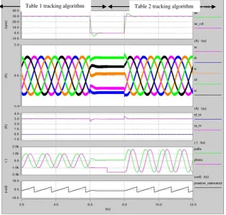
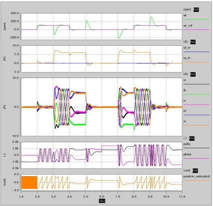
The results shown in figure 9 demonstrate the validity of the saliency tracking algorithms. The motor was working at 120 rpm speed and at half load. At t=2s a speed step change from 120 rpm to 0 rpm was applied to the system. Then at t=3 s another speed step change from 0 rpm to -120 rpm was introduced to the system. After that at t=5 s a zero speed was applied to the system and finally at t=6s a speed step change from 0 rpm to 120 rpm was applied to the system. The algorithm that is used to track the saliency from the begging to t= 4s is the one given in table 1 (using V1,V4 and V0) while the algorithm given in table 2 (using V2,V3 and V0) is used to track the saliency for the rest of the test. The results show that the motor responded to the load and speed steps very fast and the proposed algorithms could track the saturation saliency (2*fe) at positive and negative speeds and more importantly at low and zero speeds. Finally, the position scalars Pa,Pb,Pc,Pd and Pe obtained from the algorithm given in table 2 has higher amplitude compared to those obtained from the algorithm given in table 1 and hence it can be said that first advantage of using the algorithm given in table 2 over using the algorithm given in table 1 is the higher signal to noise ratio. 3.2 Fully Sensorless Speed Control

The speed control for a five-phase PM machine drive has been implemented in simulation in the Saber modeling environment. This estimated speed 𝜔𝑟^ and position 𝜃𝑟^are used to obtain a fully sensorless

(8)

PI

d1 q1 d3 q3

a b c d e

Multiphase SVPWM

PMSM d/dt

Id1_ref=0 Vd1_ref

Vq1_ref

wr_ref Iq1_ref

Ia

Ib

Ic Va_ref

Vb_ref

Vc_ref

Vd_ref

Ve_ref PI

Id3_ref=0

PI Iq3_ref=0

Vd3_ref

Vq3_ref

d1 q1 d3 q3

a b c d e

Id

Ie

Mechanical observer

d

ia

/d

t

Estimated_position Kt

d

ib

/d

t

d

ic

/d

t

d

id

/d

t

d

ie

/d

[image:8.595.118.480.102.727.2]

t

Figure 8 saliency tracking control topology for five phase drive

Figur 9 . saliency tracking results

(9)

PI

PI d1_q1

d3 q3

a b c d e

Multiphase SVPWM

PMSM

d/dt

Id1_ref=0 Vd1_ref

Vq1_ref

wr_ref Iq1_ref

Ia

Ib

Ic Va_ref

Vb_ref

Vc_ref

Vd_ref

Ve_ref

PI

Id3_ref=0

PI

Iq3_ref=0

Vd3_ref

Vq3_ref

d1 q1 d3 q3

a b c d e Id_Ie

Mechanical observer

d

ia

/d

t

θr^

Kt

d

ib

/d

t

d

ic

/d

t

d

id

/d

t

d

ie

/d

t

ωr^

[image:9.595.166.431.84.272.2]

Figure10. the sensorless vector control structure for the five-phase inverter PMSM drive

[image:9.595.133.462.380.691.2]

Figure 11 shows the results of a fully sensorless speed control of a five phase PMSM motor driven by a five phase inverter at a half load condition using the algorithms presented in this paper. The motor was working in sensorless mode at speed = 1 Hz then at t=6 s a speed step change from 1 Hz to 0 rpm (till t=8 s) is applied to the system. The algorithm given in table 1 is used to track the saliency from the begging till t= 7s then the algorithm given in table 2 is used for the rest of the test. Figure 11 shows that the motor responded to the speed step with a good transient and steady state response regardless of which algorithm to track the saliency is used.

Figure 11 Fully Sensorless Speed Steps between 0.5 Hz,0 to 0.5 Hz at half load.

Figure 12 demonstrate the stability of the fully sensorless system when a load disturbance where applied. The motor was working at zero speed and at no load in sensorless mode. Then a step change from 0 rpm to 100 rpm is applied to the system at t=2 s. After that a full load step is applied to the motor at t=3 s. At t=5s

(10)

[image:10.595.84.513.162.576.2]

a speed step change from 100 rpm to 0 rpm is applied to the system. Then at t=5 s the motor became unloaded. After the at t= 7s a full load step is applied again to the system. At t= 8s a speed step change from 0 rpm to 100 rpm is applied to the system. After that at t= 9s the motor became unloaded again. Finally at t=10s a speed step change from 100 rpm to zero is applied to the system. The algorithm given in table 1 is used to track the saliency from the begging till t= 7s then the algorithm given in table 2 is used for the rest of the test. The results shows that the system maintained the speed in all the cases.

Figure 12 Fully Sensorless full load Steps.

3.3 Current Distortion reduction

(11)

A

B

C

D

E

T0/2 T1/2 T2/2 T3/2 T4/2 T0/2

00000 10000 11000 11001 11101 11111

tmin

A

B

C

D

E

T0/2T1/2 T2/2T3/2 T4/2 T0/2

00000 10000 11000 11001 11101 11111

[image:11.595.91.511.88.197.2]

tmin tmin

Fig 13 Space vector modulation state diagram for five phase inverter in case that V_ref_α1-β1 exists in first sector a) V1 and V4 are extended as in table 1, b) V2 and V3 are extended as in table 2.

The time duration (T0,T1,T2,T3 and T4) of the active vectors shown in fig 13.a and 13.b are obtained using equations (7-9). It should be highlighted that when the phase voltage is sinusoidal, or the magnitude of the d3q3– axes voltage vector is zero as in our case, the following equations hold true [12]:-

𝑇3 = 1.618 ∗ 𝑇1….(42)

𝑇2 = 1.618 ∗ 𝑇4 ….(43)

This means that the extension of the vectors V2 and V3 will be less than that of the vectors V1 and V4 which helps to reduce the current distortion introduced to the motor stator currents as shown in fig 14.a fig 14.b and fig 14.c. Fig 14.a demonstrate the sequence of applying the active vectors V1,V2,V3,V4 to generate the reference voltage Vref_α1-β1 if it exists in the first sector in the normal case (without extensions). In Fig 14 b the active vectors V1 and V4 are extended to tmin and finally in fig 14.c the active V2 and V3 are extended to tmin. From the figures it is quite clear that the voltage ripples (grey areas) in the case of extending the active vectors V2 and V3 is less than those in the case of extending the active vectors V1 and V4 and so less current distortion will be introduced to the motor stator currents.

sector1 sector1

sector1 (01000)

(10100)

(11010) (11101)

(11000)

(11001) (10000)

(01001) Phase a Vref_α1-β1

V1

V2

V3

V4

V3

V2

V1

(01000)

(10100)

(11010) (11101)

(11000)

(11001) (10000)

V1

V2

V3 V4

V4

V3

V2

V1

(01000)

(10100)

(11010) (11101)

(11000)

(11001) (10000)

V1

V2

V3

V4

V3

V2

V1

Fig 14 a

Fig 14 b

[image:11.595.92.506.387.554.2]

Fig 14 c

Fig 14. Current ripple for different extension schemes. a) no extensions. b) extension of active vectors V1 and V4. c) extension of active vectors V2 and V3.

(12)

[image:12.595.122.478.83.637.2]

Fig 15 current waveform under different extension schemes

(13)

[image:13.595.130.472.94.258.2]

Fig 16 FFT of the current waveform under different extension schemes. a) no extensions b) extension of active

vectors V1 and V4 c) extension of vectors V2 and V3.

4. Conclusion

This paper has outlined a two new algorithms for tracking the saliency of motor fed by a five-leg inverter in through measuring the dynamic current response of the motor line currents due the IGBT switching actions. The proposed methods include software modification to the method proposed in[18] to track the saliency of the motor fed by three phase inverter . The two new algorithms can be used to track the saturation saliency in PM and the rotor slotting saliency in induction motors. The results have shown the advantages of using the switching action of the active vectors V2 and V3 over using the active vectors V1 and V4 in terms of quality of the estimated position signals and the distortion introduced to the stator currents by extending the narrow vectors.

References

[1] Villani M, Tursini M, Fabri G, Castellini L. Multi-phase fault tolerant drives for aircraft applications. In: IEEE 2010 Electrical Systems for Aircraft, Railway and Ship Propulsion Conference (ESARS); 19-21 October 2010; Bologna, Italy. New York, NY, USA: IEEE. pp. 1–6.

[2] Qingguo S, Xiaofeng Z, Fei Y, Chengsheng Z. Research on space vector PWM of five-phase three-level inverter. In: IEEE 2005 Electrical Machines and Systems conference (ICEMS); 29-29 September 2005; Nanjing, China. New York, NY, USA: IEEE. pp. 1418-1421.

[3] Ruhe S, Toliyat HA. Vector control of five-phase synchronous reluctance motor with space vector pulse width modulation (SVPWM) for minimum switching losses. In: IEEE 2002 Applied Power Electronics Conference and Exposition (APEC);10-14 March 2002; Dallas, Texas, USA. New York, NY, USA: IEEE. pp. 57-63.

[4]Abbas MA, Christen R, Jahns T.M. Six-phase voltage source inverter driven Induction motor. IEEE T Ind Appl 1984; 20: 1251-1259.

[5] Zhao X, Lipo TA. Space vector PWM control of dual three-phase induction machine using vector space decomposition. IEEE T Ind Appl 1995; 31:1177-1184.

[6] Parsa L, Toliyat HA. Multi-phase permanent magnet motor drives. In: IEEE 2003 Industry Applications Conference (IAS); 12-16 October 2003; Utah, USA. New York, NY, USA: IEEE. pp. 401-408.

[7] Xu H, Toliyat HA, Pertersen LJ. Five-phase induction motor drives with DSP-based control system. IEEE T Ind Appl 2002; 17: 524-533.

[8] Kelly JW, Strangas EG, Miller JM. Multiphase space vector pulse width modulation. IEEE T Energy Conver 2003; 18: 259-264.

[9] Xue S, Wen X, Feng Z. A novel multi-dimensional SVPWM strategy of multiphase motor drives. In: EPE 2006 Power Electronics and Motion Control Conference; 30 August- 1 September 2006; Portoroz, Slovenia. Brigitte Sneyers, Pleinlaan 2, Brussels, Belgium: EPE. pp.931-935.

[10] Pengfei W, Ping Z, Fan W, Jiawei Z, Tiecai L. Research on dual-plane vector control of five phase fault-tolerant permanent magnet machine. In: IEEE 2014 Transportation Electrification Asia-Pacific conference (ITEC Asia-Pacific); 31 August- 3 September 2014; Beijing, China. New York, NY, USA: IEEE. pp. 1-5.

(14)

[11] Minghao T, Wei H, Ming C. A novel space vector modulation strategy for a five-phase flux-switching permanent magnet motor drive system. In: IEEE 2014 Electrical Machines and Systems conference (ICEMS); 22-25 October 2014; Hangzhou, China. New York, NY, USA: IEEE. pp.1622-1628.

[12] Keng-Yuan Chen. Multiphase pulse-width modulation considering reference order for sinusoidal wave production. In: IEEE 2015 Industrial Electronics and Applications conference (ICIEA); 15-17 June 2015; New Zealand, Auckland. New York, NY, USA: IEEE. pp.1155-1160.

[13 ] Z.M.S.El-Barbary. DSP Based Vector Control of Five-Phase Induction Motor Using Fuzzy Logic Control. International Journal of Power Electronics and Drive System (IJPEDS) Vol.2, No.2, June 2012, pp. 192~202

[14] Atif Iqbal, Shaikh Moinoddin*, Khaliqur Rahman. Finite State Predictive Current and Common Mode Voltage Control of a Seven-phase Voltage Source Inverter. International Journal of Power Electronics and Drive System (IJPEDS) Vol. 6, No. 3, September 2015, pp. 459~476

[15] Olivieri C, Fabri G, Tursini M. Sensorless control of five-phase brushless DC motors. In: IEEE 2010 Sensorless Control for Electrical Drives conference (SLED); 9-10 July 2010; Padova, Italy. NewYork, NY, USA: IEEE. pp.42-31.

[16] Karampuri R, Prieto J, Barrero F, Jain S. Extension of the DTC technique to multiphase induction motor drives using any odd number of phases. In: IEEE 2014 Vehicle Power and Propulsion Conference (VPPC); 27-30 October 2014; Coimbra, Portugal. NewYork, NY, USA: IEEE. pp.1-6.

[17] Parsa L, Toliyat HA. Sensorless direct torque control of five-phase interior permanent-magnet motor drives. IEEE T Ind Appl 2007; 43: 952 – 959.

[18] wubin K, Jin H, Ming K, Bingnan L. Research of sensorless control for multiphase induction motor based on high frequency injection signal technique. In: IEEE 2011 Electrical Machines and Systems conference (ICEMS); 20-23 August 2011; Beijing, China. NewYork, NY, USA: IEEE. pp.1-5.

[19] Minglei G, Ogasawara S, Takemoto M. An inductance estimation method for sensorless IPMSM drives based on multiphase SVPWM. In: IEEE 2013 Future Energy Electronics Conference (IFEEC); 3-6 November 2013; Tainan, Taiwan. NewYork, NY, USA: IEEE. pp.646-651.

[20] Schroedl M. Sensorless control of AC machines at low speed and standstill based on the INFORM method. In: IEEE 1996 Industry Applications Conference; 6 -10 October 1996; San Diego, USA. New York, NY, USA: IEEE. pp. 270-277.

[21] Holtz J, Juliet J. Sensorless acquisition of the rotor position angle of induction motors with arbitrary stator winding. In:IEEE 2004 Industry Applications Conference; 3-7 October 2004;Washington, USA. NewYork, NY, USA: IEEE. pp.1321-1328.

[22] Qiang G, Asher GM, Sumner M, Makys P. Position estimation of AC machines at all frequencies using only space vector PWM based excitation. In: IET 2006 International Conference on Power Electronics, Machines and Drives; 4-6 April 2006; Dublin, Ireland. Savoy Place, London, UK: IET.pp. 61-70.

[23] Lorenz RD, Van Patten KW. High-resolution velocity estimation for all-digital, ac servo drives. IEEE T Ind Appl 1991;27:701–705

[24] Y. Hua, M. Sumner, G. Asher, Q. Gao and K. Saleh, "Improved sensorless control of a permanent magnet machine using fundamental pulse width modulation excitation," in IET Electric Power