Extraction of synaptic input properties in vivo

Extraction of synaptic input properties

in vivo

Paolo Puggioni

_{, Marta Jelitai}

_{, Ian Duguid}

_{and Mark C.W. van Rossum}

May 6, 2016

1_{Neuroinformatics Doctoral training Centre, School of Informatics, University of Edinburgh}

2_{Institute for Adaptive and Neural Computation, School of Informatics, University of}

Edin-burgh, 10 Crichton Street, Edinburgh EH8 9AB, UK

3_{Centre for Integrative Physiology, University of Edinburgh, Hugh Robson Building,}

Edin-burgh EH8 9XD, UK

4_{Presently at Institute of Experimental Medicine of the Hungarian Academy of Sciences,}

Budapest, Hungary.

Abstract

Knowledge of synaptic input is crucial to understand synaptic integration and ultimately neural

function. However, in vivo the rates at which synaptic inputs arrive are high, that it is typically impossible to detect single events. We show here that it is nevertheless possible to extract the

properties of the events, and particular to extract the event rate, the synaptic time-constants, and the properties of the event size distribution fromin vivovoltage-clamp recordings. Applied to cerebellar interneurons our method reveals that the synaptic input rate increases from 600Hz during rest to 1000Hz during locomotion, while the amplitude and shape of the synaptic events are unaffected by

this state change. This method thus complements existing methods to measure neural functionin vivo.

Significance Statement

Neurons in vivo typically receive thousands of synaptic events per second. While methods have been

developed to measure the total synaptic current that results from these events, extraction of the

con-stituent events has proven very difficult given their high degree of overlap. To resolve this, we introduce

a probabilistic method that extracts the statistics of synaptic event amplitudes and their frequency from

voltage clamp recordings, which is then applied to recordings from cerebellar interneurons. With this

method it becomes possible to better understand synaptic input and how it changes with behavioral

Introduction

Neurons typically receive a barrage of thousands of excitatory and inhibitory events per second. As

these inputs determine to a large extent the spiking activity of the neuron, it is important to know the

properties of synaptic input and how it changes, for example, with behavioral state (e.g. sleep, attention,

locomotion), with plasticity, or with homoeostasis. Consider a neuron receiving synaptic input while the

total current is being measured in voltage-clamp, Fig.1a. While in vitro, or in cases where activity is artificially lowered, individual excitatory and inhibitory inputs can be resolved (top), in vivo the rates

are typically so high that this is impossible. Instead, the total synaptic current trace is wildly fluctuating

and single event extraction methods will fail.

Nevertheless, information can still be extracted from the statistical properties of the recorded in

vivo currents. This study is based on the fact that although individual synaptic events might not be distinguishable in the observed current trace, the trace will still bear signatures of the underlying events.

Intuitively, the mean current should be proportional to the product of the synaptic event size and the

total event frequency. But it is possible to extract other information as well. For instance, when the

synaptic events have short time-constants, the observed current trace will have more high frequency

content than when the synaptic time-constants are slow. Similarly, when the input is composed of many

small events, the variance of the current trace will be smaller than when it is composed of a few large

events. Here we introduce a method that aims to infer the event rate, synaptic time-constants, and

distribution of synaptic event amplitudes from the power spectral density and statistical moments of the

observed current trace.

We applied our method to voltage-clamp traces of electrotonically compact interneurons recorded

in the cerebellum of awake mice. We find that during voluntary locomotion, the excitatory input rate

increases from 600 to 1000 Hz, while the synaptic event amplitudes remain the same. Our method thus

provides a novel way to resolve synaptic event propertiesin vivo.

Methods

We implemented the model in PyMC, a python package to perform Bayesian computation (Patil, Huard,

and Fonnesbeck, 2010), using a Metropolis Hastings sampler, with normal proposal distribution and

standard deviation in each dimension equal to 1 over the absolute value of the parameters. Usually, the

auto-correlation of the chains was about 300−500 samples and the burn-in phase was about 10 effective samples. To construct the posterior, we generated 150,00 samples yielding∼400 effective samples and assessed the mixing by using the Geweke method provided by the PyMC package. The computational

analysis tools and data are available atwww.to_be_announced.org.

To compare our method to traditional single event detection methods, we employed TaroTools, a freely

available IgorPro package (see sites.google.com/site/tarotoolsregister/) to detect putative post-synaptic

currents (PSCs).

The experimental data is described in detail elsewhere. Briefly, whole-cell patch clamp recordings of

a

Arrival times

2 ms τ

1 _τ

2 a

Voltage clamp trace

in vitro- like

in vivo - like

Synaptic inputs

20 ms

EPSC

b

Figure 1. Inference of synaptic properties. a) A neuron receives input from a number of synapses under a Poisson rate assumption. The events have identical shape, but the amplitudeavaries between events. Right: Forin vitro experiments synaptic events rates are typically low and the individual events can be extracted and quantified. However, forin vivo experiments, rates are high and individual events are not distinguishable. b) Analysis based on semi-automated single event extraction produces incorrect results when the total rate exceeds 500 HZ. From left to right: estimated event frequency, estimated mean event amplitude, estimated standard deviation of the event amplitude. Model parameters:

ak = 50pA. rise-timeτ1= 0.3 ms and the decay-timeτ2= 2 ms.

of 100-300 µm from the pial surface of the cerebellum, using a Multiclamp 700B amplifier (Molecular

Devices, USA). The signal was filtered at 6 - 10 kHz and acquired at 10 - 20 kHz using PClamp 10 software

in conjunction with a DigiData 1440 DAC interface (Molecular Devices). Patch pipettes (5-8 MΩ) were

filled with internal solution (285-295 mOsm) containing (in mM): 135 K-gluconate, 7 KCl, 10 HEPES, 10

sodium phosphocreatine, 2 MgATP, 2 Na2ATP, 0.5 Na2GTP and 1 mg/ml biocytin (pH adjusted to 7.2

with KOH). External solution contained (in mM): 150 NaCl, 2.5 KCl, 10 HEPES, 1.5 CaCl2, 1 MgCl2

(adjusted to pH 7.3 with NaOH).

To detect movement, the animals were filmed using a moderate frame rate digital camera (60 fps)

synchronized with the electrophysiological recording. We defined a region of interest (ROI) covering the

forepaws, trunk and face and calculated a motion index between successive frames (as in Schiemann et

Results

A common method to extract synaptic properties is to identify and analyze isolated events from current

traces, butin vivothis fails because the events will overlap, Fig.1a. To demonstrate the problem explicitly

we simulated a neuron randomly receiving excitatory synaptic events (see below for model details). For

illustration purposes we assume momentarily that the amplitude of all events is identical (50pA). From

the total current recorded in voltage clamp we attempt to reconstruct the frequency of events and the

distribution of their amplitudes.

We used single event dectection software (see Methods) to find putative post-synaptic currents (PSCs).

At low input frequencies (50Hz), most of PSCs were correctly identified and the resulting estimation of the

synaptic input amplitude distribution was correct. However, at higher frequencies, when the event interval

became shorter than the synaptic decay time, the event frequency was grossly underestimated and reached

a plateau, Fig. 1b, left. At this point the individual EPSCs overlapped and became indistinguishable.

The reason is that the most probable inter-time interval of a Poisson process (a common model for the

inputs received by a neuron, but see Lindner, 2006) is zero. In addition, as a result of the overlap, the

estimated PSC amplitude distribution had peaks at multiples of the original amplitude and the variance

of the event amplitude was highly overestimated, Fig. 1b right. Finally, at high input frequencies the

traces had to be manually post-processed to correct mistakes in event detection. This manual processing

is time consuming - even an experienced researcher spent more than 1 hour to analyze a 10 second trace.

Thus at high input frequencies single event analysis is not only incorrect, it is also time consuming.

Generative model for the observed current trace

Unlike thein vitro situation, the synaptic properties are not directly accessible fromin vivo recordings.

Instead, the data indirectly and stochastically reflects the synaptic properties. We therefore use a

gener-ative model to couple the data, in particular the statistics of the current trace, to the underlying synaptic

properties. We define the generative model as follows: the synaptic inputs are assumed to arrive according

to a Poisson process with a rateν, Fig.1a (also see Discussion). The synaptic events are modelled with

a bi-exponential time-course as this can accurately fit most fast synapses (e.g. Roth and van Rossum,

2009)

f(t) = (1−e−t/τ1_)e−t/τ2 _{(t >0) (1)}

While we initially assumed that all PSCs have the same time constants, the effect of heterogeneous

time-constants is studied below. The total current is

I(t) =

K

X

k=1

akf(t−tk), (2)

wheretkdenotes the time of eventk, andakis the amplitude of that event. Unlike the schematic example

above, the event amplitudes were drawn from a synaptic amplitude distributionP(a) (witha≥0). This distribution captures the spread of amplitudes across the population of synapses, as well as variation in

Although our method is general and not restricted to any specific distribution of synaptic amplitudes,

we consider for concreteness the amplitudes to be distributed as either: 1) a log-normal distribution

(LN)

P(a) = 1

p2 √

2πae

−(lna−p1 )2

2p2

p _{, (3)}

with raw moments an _≡´∞

0 P(a)a

n_da=enp1+n2p22/2. Or, 2) a stretched exponential distribution (SE)

P(a) = 1

p1Γ(1 + 1/p2)

e−(a/p1)p2_{, (4)}

with moments an ₌ p n

1

p2

Γ ((1 +n)/p2)/Γ(1 + 1/p2) where Γ(·) is the Gamma function. Or, 3) a

zero-truncated-normal distribution (TN)

P(a) = φ(a/p2+h)

p2[1−Φ(h)]

, (5)

where h=−p1/p2, andφ(·) and Φ(·) are the density of a normal distribution with zero-mean and unit

variance and its cumulative. The mean µa =p1+p2ρand variance σa2=p22−p22(ρ2−ρh)−µ2a, where

ρ=φ(h)/[1−Φ(h)] (for higher moments see Horrace, 2013).

The stretched exponential distribution has a maximum at zero amplitude, while the two other

dis-tributions have an adjustable mode that is non-zero, but differ in the heaviness of their tails. The LN

and SE are heavy-tailed, while the TN distribution is not. These three probability distributions are commonly used in the experimental and theoretical literature (Song et al., 2005; Barbour et al., 2007;

Buzs´aki and Mizuseki, 2014). Note that while conveniently all these distributions are characterized by

the two parametersp1andp2, which determine the mean and variance of the distribution, the parameters

themselves are not comparable across distributions.

Moments of the synaptic current

Next, we calculated the current trace I(t) that results from the random inputs. The statistics of the

current follow from the distribution of synaptic event amplitudes and the time-course of the events

according to Campbell’s theorem (Rice, 1954; Bendat and Piersol, 1966; Ashmore and Falk, 1982). The

cumulants κn of the current probability distribution P(I) follow from the event distribution and the

synaptic time-course as

κn=νan

ˆ ∞

0

[f(t)]ndt, (6)

In this equation the raw momentsan _{of the synaptic event amplitude distributionP(a), are given above}

for the different candidate distributions. Furthermore, for the bi-exponential synaptic kernelf(t) (Eq. 1)

the integrals are´₀∞[f(t)]n_dt=n!τ

1Γ(nτ_τ1

2)/Γ(1 +n+n

τ1

are expressed in the cumulantsκn. In practice we use the first four moments of the current distribution,

µI =κ1

σI =

√ κ2

skew(I) =κ3/κ 3/2 2

kurtosis(I) = (κ4+ 3κ2)/κ22−3.

(7)

We can thus express the statistical moments of the distribution of the observed current trace, Eq.7, in

the underlying model.

Power spectrum of the synaptic current

Also the power spectral density (PSD) of the current I(t) can be expressed in the model parameters

(Puggioni, 2015). The current is the convolution a Poisson process, which has a flat power spectrum,

with the synaptic kernel. As a result the PSD is the magnitude of the Fourier transform of the synaptic

kernel and for non-zero frequencies equals

PSD(f) = 2ν(µ2_a+σ2_a) τ

4 2

(τ1+τ2)2+ (2πf τ2)2(2τ12+ 2τ1τ2+τ22) + (2πf τ2)4τ12

. (8)

Note that being a second order statistic, the PSD depends on the mean and variance of the amplitude

distributionP(a) only.

Inference procedure

Now that we have expressed both the PSD and the moments of the current distribution in the model

parameters, one could proceed using classical fitting techniques, such as least square fitting, to find the

synaptic parameters that best fit the data. However, we use a probabilistic approach that yields the

distributionof parameters that best fit the data. A probabilistic approach is advantageous because 1) we expect strong correlations between the model parameters, 2) the probabilistic approach naturally yields

the probability distribution of possible fit parameters, and 3) the probabilistic model is straightforwardly

extended to include a variety of experimental effects that are crucial in describing the data.

However, before including these we first present an idealized model, which ignores some distortions

typical ofin vivorecordings. Fig. 2 shows the Bayesian network and the dependencies among the variables (nodes). The green nodes stand for variables that are measured directly from the data: the PSD and

the first four moments of the current MI = [µI, σI,skewI,kurtosisI]. Together the data are succinctly

denotedD. The orange nodes represent variables that are to be inferred. The 5 parameters of the model

are the rateν, the mean synaptic amplitudeµa, its varianceσa, synaptic rise-timeτ1and decay timeτ2,

a _a Power

Spectrum

M_a Syn. event

std σ {LN, SE, TN} Weight distribution

M_I Observed current

moments

Current (pA)

Synaptic event moments

H

Low freq noise σ

L

Hi freq noise σ

Syn. event mean µ

0

Baseline current I

1 Syn. rise

time τ

2

Syn. decay time τ

Event rate ν

Figure 2. Bayesian network representing the dependencies between the variables. Orange nodes represent variables that have to be inferred from the data, green nodes stand for variables that are measured directly from the data. The blue nodes are additional contributions to the current in typical experiments. The top left graph shows the PSD fit (red line is the fit with Eq. 8) and the bottom right graph is the probability distribution ofI(t), used to calculate the observed momentsMI. All variables

are described in Table 1.

Written formally, the joint probability of the Bayesian network in Fig. 2 is

Pjoint(θ,D) =P(τ1|PSD)P(τ2|PSD)P(Ma|µa, σa, Sa)×

P(µa)P(σa)P(ν)P(MI|τ1, τ2, Ma, ν)

(9)

From this the parameter distribution given the data P(θ|D) follows as P(θ|D) ∝ Pjoint(θ,D). We

now describe Pjoint and the probabilistic dependencies among the nodes term by term. The first two

terms infer the values for the synaptic time-constants from the PSD. Since we cannot obtain an analytic

expression of the likelihood of the PSD, we use empirical Bayes to set the prior on the time constants of

the post-synaptic current (Casella, 1985). We fit Eq. 8 with a least square method to the PSD to findτ1

andτ2(see top left inset in Fig. 2). Since we found the cross terms of the Hessian matrix betweenτ1and

τ2to be very small (<0.005), we model the time constants with independent Gaussian distributions with

mean and variance given by the mean and the Hessian of the PSD fit. A common criticism of empirical

Bayes is that it uses data for both prior and inference, thus double counting the data. Here however, the

PSD data is used to set the prior on the time constants, but it is not used as evidence in the inference

process, Fig. 2.

The next term in Eq. 9 isP(Ma|µa, σa, Sa). This is a deterministic function, because the moments

of the synaptic amplitude distribution Ma are fully determined by µa, σa and the type of amplitude

distribution type, see Eqs. 3-5. The parameters µa, σa and ν are given uninformative uniform priors

spanning a reasonable and positive range of values.

Parameter name Description

Measured dataD

MI = (µI, σI,skewI,kurtosisI) Observed first four moments of the currentI(t)

P SD Power spectral density of I(t)

Parameter of idealized model τ1,τ2 Rise and decay time of the EPSCs

Sa={LN,SE,TN} Synaptic amplitude distribution =

{log-normal, stretched exponential, truncated normal} µa,σa Mean and std. of the amplitude distribution

Ma Moments of the synaptic amplitude distribution

ν Frequency of synaptic inputs

Additional parameters of full model i0 Voltage clamp baseline current

σH Std. of high frequency noise

σL Std. of low frequency fluctuations

Table 1. Description of the parameters and variables of the model.

calculated analytically. Although Eq. 6 gives the expected value,MI is a stochastic quantity that due to

the Poisson process is different on each run and thus requires simulation. However, below we present a

method to speed up its calculation.

Inclusion of in vivo variability and other experimental confounds

In vivo voltage clamp recordings show a number of effects that need to be included in the model via additional parameters. The first additional feature is the baseline current (i0) of the voltage clamp that

has to be subtracted from the current. In in vitro situations one can estimate it by finding the baseline of the current trace, but due to the high rates this is challenging for in vivo recordings. Instead a prior

probability of P(i0) was included. It was normally distributed with mean and variance estimated with

an informed guess, reflecting the uncertainty in the value ofi0.

The second feature is the inclusion of high frequency noise coming from the recording set-up and

for instance the stochastic opening and closing of ion channels. Its standard deviation σH is measured

experimentally and we model it as a zero mean Orstein-Uhlenbeck (OU) process

dUHt =−τHUHtdt+σH p

2/τHdBt, (10)

whereBtis a Wiener process and the cut-off frequency is 1/(2πτH) = 600 Hz.

Finally we include low frequency fluctuations typically present inin vivosynaptic activity (e.g. Schie-mann et al., 2015). We relax the constant rate assumption by adding a modulation term to the Poisson

rate, which is modeled as an OU process with powerσ2_Land cut-off frequencyfL = 1/(2πτL) of 5 Hz

dULt =−τLULtdt+σL p

+

+

+

+

+

+

+

2

6

4

8

1.2

1.6

1.4

1.8

23

25

24

26

Std (pA)

Skewness (pA)

Kurtosis (pA)

31 32 33 34 23 24 25 26 1.2 1.4 1.6 1.8

Mean (pA) Std (pA) Skewness (pA)

Likelihood of the moments of the synaptic current

Figure 3. Likelihood of the moments of the synaptic currentP(MI|τ1, τ2, Ma, ν) as estimated by

simulating the generative model multiple times with fixed parameters τ1, τ2, Ma, ν. Red crosses

represent the analytic predictions of the expected values of theMI.

As a result in the expression for the PSD, Eq. 8, the rate ν is replaced by (ν+P SDOU(f)), where the

power spectrum of the OU process is given byP SDOU(f) =σ2LτL/[1 + (2πf τL)2]. To find the variance of

this slow noise, we fit the PSD with Eq.8 in a range abovefLand calculate its integralσth(the theoretical

standard deviation of the modulation-free trace). Since the observed variance of the signal σ_obs2 is the

sum of σ2

th and σL2 (the slow component is independent from the underlying process), it follows that

σ2

L=σ

2

obs−σ

2

th.

These three additional features are depicted by the blue nodes in Fig. 2. The joint probability becomes

for the full model

Pjoint=P(τ1|PSD)P(τ2|PSD)P(Ma|µa, σa,Sa)P(µa)P(σa)P(ν)×

P(i0)P(σH)P(σL|PSD)P(MI|τ1, τ2, Ma, ν, i0, σH, σL)

(12)

Description of the sampling algorithm

In the Bayesian framework, the posterior probabilities of the parameters of the model can be estimated

by sampling from Pjoint, for instance using a suitable Markov chain Monte Carlo algorithm. However,

this approach is very slow, because the likelihood does not have a closed form and has to be estimated

with multiple simulations after each MCMC sample. As the estimation of the likelihood takes about 1

We introduce a speed up that can be used whenever a likelihood can only be obtained by sampling from

the generative model, but its means can be calculated analytically. The idea is to fit the likelihood with a

kernel density estimate (KDE). Assuming that the shape of the likelihood does not depend much on the

parameter values, the same KDE can be exploited to approximate the likelihood for different parameter

values. As a result we can keep the shape fixed, but we translate it to a new location determined by the

analytically calculated average moments of the likelihood. A thorough validation shows that the method

correctly infers the parameters across a wide range of biologically plausible values (see below).

To perform the inference, we first initialize the parameters{τ1, τ2, Ma, ν}by Least-Square fitting Eq. 7

to the observed moments and Eq. 8 to the observed PSD. Next, we run the generative model multiple

times to calculate the shape of P(MI|τ1, τ2, Ma, ν) using an exponential KDE. Finally, during the main

MCMC run where we sample Pjoint, we keep the shape fixed but at each step we translate it to the

location of the analytically calculated average moments (Eq. 6, red crosses in Fig 3).

Validation on simulated data

a

30 45 60 6 12 18 24

6

12

18

24

300

450

600

b

σa

(pA)

σa

(pA)

µa(pA)

µa(pA)

σ

a(pA)

σ

a(pA)

ν

(Hz)

ν

(Hz)

ν

µa

(pA)

^

^

^

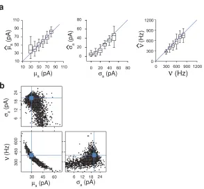
Figure 4. Validation of the method on simulated data.

a) The inference gives good results in a physiological range of parameters. True (x-axis) vs estimated parameters. The boxes represent the 33rd_{and 66}th _{quantile of the distributions, the whiskers indicate}

the full range. The distribution of synaptic amplitudes was Log-Normal.

b) Inferred distribution of model parameters across multiple trials generated with fixed parameters (blue markers).

inference method to recover their values. One parameter at a time was varied while the other parameters

were set to a default value (µa = 50 pA, σa = 40 pA, ν = 700 Hz). We first assumed that the shape of

the synaptic amplitude distribution (LN, SE, orTN) isa priori known. Fig. 4a compares the estimated parameters vs. their true value. The inference works well in a physiologically plausible range and the

true value is almost always within the confidence interval. The largest error bars occur when either the

mean event amplitude is small or the std dev. is large, i.e. the CoV is large.

The approach also yields the inferred joint distribution for a given parameter setting. The posterior

distribution of the parameters contains the true values in the region of maximal density, Fig. 4b. Unlike

single point estimates (e.g. maximum a posteriori, MAP estimates), one can also evaluate the

depen-dencies between the parameters. In particular we observe a strong anti-correlation between event rate

and event size (bottom left panel). In other words, the model compensates for changes in the rate by

changing the estimate for the event size; their product is approximately invariant.

Model selection

Next, we tested whether the method is able to recover the correct amplitude distribution (LN, SE, or, TN) when it is not knowna priori. The Bayesian framework offers straightforward tools to assess the

likelihood of a model, such as the Deviance Information Criterion (DIC) (Spiegelhalter et al., 2002). The

higher is the DIC, the less likely is the model suitable to describe the data, and this would be the simplest

way to choose the most likely distribution. However, the DIC value is a random variable that varies from

trial to trial. Thus rather than selecting the lowest DIC, we use Bayesian model comparison based on

the distribution of the DIC values. We generated 100 traces using a given amplitude distribution and

run the inference algorithm assuming either LN, SE, or TN amplitude distribution and we calculate the DIC for each mode, Fig. 5a. From the three DIC values of the three models DICLN, DICSE,

and DICT N (corresponding to the LN, SE, and TN model respectively) we calculate two quantities:

∆LT = DICLN−DICT N, and ∆LE = DICLN−DICSE. To find the most likely amplitude distribution,

we apply Bayes theorem and calculate

P(X|∆LE,∆LT) =

P(∆LE,∆LT|X)P(X)

ΣY∈[LN, T N, SE]P(∆LE,∆LT|Y)P(Y)

,

= P(∆LE,∆LT|X) ΣY∈[LN T N, SE]P(∆LE,∆LT|Y)

,

(13)

where in the second line we assumed that each amplitude distribution is a priori equi-probable. Thus, for each point in the space (∆LE,∆LT), we select the distribution which has the highest probability

according to Eq.13, see Fig. 5b. This method is able to correctly identify the amplitude distribution with

∼90% accuracy, Fig. 5c.

Robustness of method

We examined the robustness of the method in a number of ways. First, we explored how the posterior

TruncNormal

Exponential LogNormal

a

b

c

Figure 5. Inference of the underlying weight distribution of simulated data. a) The distribution of DIC differences for the three simulation weight distributions. As the shapes of the distributions differ, we used Bayesian model selection. b) The resulting maximum likelihood solution that tells which underlying distribution is most likely. c) Performance of the algorithm to recover the correct weight distribution (expressed as fraction correct, based on 100 runs).

yield narrower, more precise distributions, because more statistics are collected. However, short intervals

are preferable, because they allow the analysis of shorter periods in in vivo traces and allows one to see more rapid modulation in the synaptic inputs. Indeed, longer traces lead to less uncertainty on the

parameters, Fig. 6a. The analysis shows that 10 second long recordings are in general enough to obtain

a reasonable estimation of the parameters.

Next, we tested what happens when we introduce variability typical ofin vivo recordings. Firstly,in

vivo activity breaks the stationary assumption of the homogeneous Poisson model and inputs typically fluctuate on a slow time scale. To test the robustness of our model, we generate in vivo-like traces

by adding an inhomogeneous component to the Poisson rate, modeled as a OU process with 5Hz

cut-off frequency. Again using simulated data, the model performs well even in presence of considerable

fluctuations in the synaptic input rate, Fig. 6b.

Finally,in vivoPSCs rise- and decay-times might vary across synapses as different synapses may have different kinetic properties and may be subject to different amounts of dendritic filtering (Williams and

Mitchell, 2008). To test whether our model performs well when the shape of the PSCs varies, the two time

constants that determine the PSC shape were independently drawn from truncated normal distributions

for each PSC. The model correctly extracted µa, σa and ν when the time-constants are heterogeneous,

a

Trace length (s)

μ

a

(pA)

σ

a

(pA)

ν

b

Low freq. modulation (%)

c

60

45

30

15

0

1000

750

500

250

0 100

75

50

25

0

^

^

^

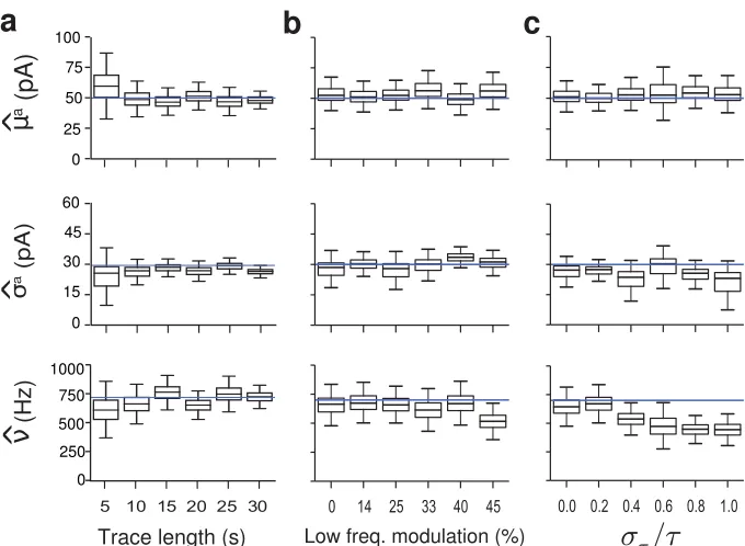
Figure 6. Robustness of inference demonstrated on simulated data. The traces were simulated with input amplitude drawn from a LogNormal distribution (µa= 50 pA, σa = 30 pA) andν= 700 Hz.

a) The estimates are robust using current traces of about 10s or longer. For shorter traces the inference is based on too little data and works less well. Top: mean single event amplitudeµa; middle: standard

deviation of amplitude; bottom: event rate.

b) Robustness toin vivo variability when an inhomogeneous low frequency (<5 Hz) component is added to the Poisson rate. The parameters’ estimation is plotted against the contribution (in percentage) of the low frequency modulation to the total standard deviation.

c) Robustness to heterogeneity in the synaptic time-constants as expressed in the CV of the rise- and decay-time constants.

Inference method applied to cerebellar

in vivo

data

We applied our inference method to in vivo recordings obtained from cerebellar interneurons. These neurons are ideal to test our method as they are electronically compact (Kondo and Marty, 1998). The

voltage clamp held neurons at -70mV to isolate excitatory inputs. The head-restrained mice displayed

bouts of self-paced voluntary locomotion on a cylindrical treadmill, Fig. 7a. All traces (n= 8) were 90

seconds long and contained at least 10 seconds of movement. Locomotion modulates subthreshold and

spiking activity in a large number of brain regions (Dombeck, Graziano, and Tank, 2009; Polack,

Fried-man, and Golshani, 2013; Schiemann et al., 2015). In cerebellar interneurons, locomotion is associated

with increased excitatory input drive, Fig. 7b. In particular we were interested in what underlies this

increased drive. For instance, it could be caused by increased frequency, increased amplitude as an effect

of neuromodulation, or recruitment of a distinct set of synapses.

sub-b

a

c

µ_a(pA)

ν_(Hz)

Pro

b.

Pro

b.

Pro

b.

Movement Quiet

d

e

ν

(Hz)

Clam

p curr

ent

Data

Infer

red

Figure 7. Analysis ofin vivo voltage-clamp recordings.

a) Experimental setup: head-fixed awake mice, walking voluntarily on a wheel. Right: Voltage clamp current in cerebellar interneurons (top) and simultaneously recorded animal movement (bottom). Periods of movement are accompanied with an increased excitatory current in the neuron. b) Left: Observed current distribution in the moving and quiet periods. Note that due to the high input frequency, periods with zero current are very rare. Right: Samples of the recorded Power Spectral Density. c) Posterior distribution of the input parameters of a representative interneuron (under Log-Normal assumption, which was the most likely distribution for this neuron). d) Inference of the synaptic input parameters across 8 recordings displaying an increase in the input frequency during movement but not in the mean or variance of the event amplitude. e) Classification of the synaptic event amplitude distribution. In both conditions both Log-normal and Stretched exponential

Quiet Movement power power to mean std err mean std err p-value of data detect 10% change

τ1 0.27 ms 0.03 ms 0.28 ms 0.03 ms 0.24 0.15 0.61

τ2 1.68 ms 0.22 ms 1.65 ms 0.19 ms 0.61 0.1 0.74

µa 42.8 pA 8.7 pA 43.2 pA 7.9 pA 1.00 0.04 0.83

σa 31.3 pA 6.2 pA 31.0 pA 4.9 pA 0.86 0.04 0.42

ν 585 Hz 153 Hz 1006 Hz 80 Hz 0.03 0.93 0.07

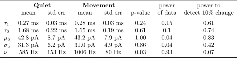
Table 2. Summary of the MAP values of the parameters estimated fromn= 8 in-vivo recordings.

sequent inference showed that the increase in excitatory synaptic current is associated with an increased

input frequency, shown for a representative trace in Fig. 7c, bottom panel. However, movement did not

lead to changes in the mean amplitude, or in the standard deviation of the synaptic amplitudes, Fig. 7c

(top and middle panels). During movement the input frequency roughly doubles, from 585 to 1006 Hz.

The synaptic time constants found by fitting the power spectrum of the current, were τ1 = 0.25±0.04

ms and τ2 = 1.56±0.21 ms (mean±standard error), comparable with the 20-80% rise time of 0.41 ±

0.14 ms and the 1.85±0.52 ms decay reported in slice (Szapiro and Barbour, 2007).

Across the population the MAP estimates ofµa, σa andν during quiet wakefulness and movement

show a similar pattern, Fig. 7d and Table 2. Note that given the small changes between quiet and moving

state, the power of the test calculated from the data is low, but 10% changes would be detected with

high probability.

Next, we applied our inference method to each trace using theLN (log-normal), SE (strechted

expo-nential),andTN (truncated normal) distribution and determined which synaptic amplitude distribution was the most likely. In general, we found that both during quiet periods and movement the most likely

distributions were heavy-tailed being either LN or SE (with exponent on average 0.8, range 0.7 - 1.2),

Fig. 7e. In particular, during active periods the LN distribution (the most common) was significantly more likely than the TN (p=0.046), but theSE distribution was not significantly less likely (p=0.37).

Thus while this suggests that the distribution is strechted, the current data can not distinguish between

theLN andSEtypes. Furthermore, we found no evidence for a change in the distribution shape between

quiet and active period (LN, p=0.78;SE, p=0.96;TN, p=0.71).

Finally, we compared our estimates to a standard single event extraction method (see Methods).

Be-cause the event extraction method fails at frequencies higher than∼500 inputs per second, the frequency of the synaptic inputs is underestimated by a factor two, due to the misclassification of overlapping events.

Discussion

In the last decade, numerous studies have been published using voltage-clamp data from anesthetized

animals to investigate the contribution of excitation and inhibition to theVmdynamics, with recordings

from auditory cortex (Wehr and Zador, 2003; Poo and Isaacson, 2009; Liu et al., 2010), visual cortex

However, in these experiments only the total excitatory or inhibitory contributions can be extracted,

therefore they are unable to distinguish properties of single synapses and changes therein. We proposed

a novel probabilistic method to infer the synaptic time-constants, the mean and variance of the synaptic

event amplitude distribution, and the synaptic event rate from in vivo voltage-clamp traces. Moreover,

the method accurately recovers the shape of the distribution of synaptic inputs. The inference is robust

to slow fluctuations of synaptic input rate, experimental noise, and to heterogeneity in the time constants

of the PSCs.

The extracted distribution reflects the amplitude of the events as received by the neuron. It therefore

includes not only variations across synapses, but also variation due to synaptic unreliability and

hetero-geneity from effects like short-term synaptic plasticity (Szapiro and Barbour, 2007). Furthermore, the

contribution of each synapse is weighted by its own input rate: synapses receiving inputs at higher rates

will contribute more to the estimated amplitude distribution than synapses receiving low rates. Our

method thus captures the effective distribution of synaptic inputs in an in vivo recording and thereby complements techniques that infer the amplitude distribution either anatomically from spine size or from

paired recordings in vitro, and that are not weighted by the input rate.

Applied to voltage-clamp recordings from cerebellar interneurons of awake mice, we found that the

excitatory synaptic amplitude distribution is either a stretched exponential or log-normal. This means

that the probability for large events is larger than for a Gaussian with same mean and variance. Such

heavy-tailed distributions have been observed in a number of systems (Sayer, Friedlander, and Redman,

1990; Song et al., 2005; Barbour et al., 2007; Ikegaya et al., 2013) and are believed to be an important

characteristic of neural processing (Koulakov, Hrom´adka, and Zador, 2009; Roxin et al., 2011;

Tera-mae, Tsubo, and Fukai, 2012). While any distribution can be tested (although for efficiency reasons the

moments should ideally be available analytically), a future goal is to reconstruct the amplitude

distribu-tion directly, for instance by reconstructing it from it moments. However, there are currently no fully

satisfactory mathematical methods to achieve this.

Furthermore we found no evidence that the synaptic amplitude distribution changes in these neurons

when the animal is moving. Instead the increase of the excitatory current during movement is due to

the higher frequency of the inputs. The most parsimonious explanation is that all inputs, big and small,

increase their rates similarly during movement. However it is important to remember that the method is

based on the ensemble of inputs. While our findings are inconsistent with a case where only large inputs

become more active, and inconsistent with a case where all single synaptic events become stronger by,

say, neuro-modulation, we can however not rule out that for instance a second population of inputs with

an identical amplitude distribution becomes active during movement.

We summarize generalizations and restrictions of the method. First, as in most methods, thein vivo

traces need to be stationary over a period long enough to accumulate sufficient statistics. The second

assumption is that synaptic inputs are uncorrelated and follow a Poisson distribution. Experimental

measurements of correlations in the brain are contradictory and largely depend on what time-scale is

considered, reviewed in Cohen and Kohn (2011). Notably, slow correlations are visible in the PSD,

adding a component with a different time-constant (Moreno-Bote, Renart, and Parga, 2008). When

that could correspond to spike correlations on time-scales_?15ms. Such correlations are included in our

model. The method would not be able to identify spike-correlations on the order of the synaptic

time-constants (τ1 andτ2), because they would contribute to the PSD in the same frequency range. However,

it is generally believed that spike count correlations on a short time scale (∼1−5ms) are small, normally

<0.03 (Smith and Kohn, 2008; Helias, Tetzlaff, and Diesmann, 2014; Grytskyy et al., 2013; Renart et

al., 2010; Ecker et al., 2010), and thus the inference would likely still give correct results.

Finally, in these population measurements truly instantaneous correlations, where multiple events

arrive simultaneously, can in principle never be distinguished from altered distributions. However, the

error associated to this effect is likely limited. Consider a neuron that receives inputs of equal amplitudea

at a rateν. If the inputs have correlationc= 0.05, it means that every 100 events, as a first approximation

one will observe on average only 95 events, 90 of sizeaand 5 of size 2a. In general, for a given correlation

c, the observed frequency isνobs=νtrue(1−c) and the observed average amplitudeaobs =atrue/(1−c).

Thus, even assumingc= 0.05, the error in the estimate would be ≤5%.

In principle, the method outlined here could be also applied to voltage-clamp recordings from

pyra-midal neurons in the cortex. However, the large size of their dendritic tree introduces space-clamp errors

(Williams and Mitchell, 2008), so that the method estimates the net conductances at the soma.Earlier

methods allow an estimation of the excitatory and inhibitory conductances using across trial average of

current injections with different magnitude (Borg-Graham, Monier, and Fr´egnac, 1996; Anderson,

Caran-dini, and Ferster, 2000; Wehr and Zador, 2003; Rudolph et al., 2004; Greenhill and Jones, 2007). More

recently, conductances have been estimated from a single trace by applying a diverse range of probabilistic

inference methods. In early studies the size of the excitatory and inhibitory inputs is assumed to be

iden-tical, fixed, and knowna priori (Kobayashi, Shinomoto, and Lansky, 2011). Moreover, synaptic inputs wereδ-functions, with instantaneous rise and decay time and Poisson statistics. Some of the assumptions

were relaxed in Paninski et al. (2012), where the number of inputs in a time window followed either an

exponential or truncated Gaussian distribution, but the synaptic decay time constant has to be known

a priori. Finally, Lankarany et al. (2013) further generalize the distribution of the number of inputs in

a time window by making use of a mixture of Gaussians. This method allows a good estimation of the

conductance traces even when the distribution of synaptic amplitudes has long tails. However, none of

these methods estimate the frequency and amplitude distribution of the input events, but instead they

recover the global excitatory and inhibitory conductances. As a result these techniques fail to distinguish

between changes in input rate, and changes in synaptic strengths.

In summary, commonly used methods to analysein vivo voltage clamp data can not infer the single event statistics at all or introduce large errors. Instead the proposed method represents an important

step to extract such information fromin vivo intracellular recordings.

Acknowledgements

We are grateful to M. Nolan, P. Latham, and L. Acerbi for helpful discussions. This work was supported

by the Engineering and Physical Sciences Research Council Doctoral Training Centre in Neuroinformatics

a Wellcome Trust Career Development fellowship (WT086602MF) to ID.

References

Anderson, J. S., M. Carandini, and D. Ferster (2000). Orientation tuning of input conductance, excitation,

and inhibition in cat primary visual cortex. J Neurophysiol84(2): 909–26.

Ashmore, J. and G. Falk (1982). An analysis of voltage noise in rod bipolar cells of the dogfish retina.

The Journal of physiology332: 273.

Barbour, B., N. Brunel, V. Hakim, and J.-P. Nadal (2007). What can we learn from synaptic weight

distributions? Trends Neurosci30(12): 622–9.

Bendat, J. and A. Piersol (1966). Measurement and analysis of random data. Wiley.

Borg-Graham, L. J., C. Monier, and Y. Fr´egnac (1996). Voltage-clamp measurement of visually-evoked

conductances with whole-cell patch recordings in primary visual cortex. J Physiol Paris90(3-4): 185–8.

Buzs´aki, G. and K. Mizuseki (2014). The log-dynamic brain: how skewed distributions affect network

operations. Nat Rev Neurosci15(4): 264–78.

Casella, G. (1985). An introduction to empirical bayes data analysis. The American Statisti-cian 39(2): 83–87.

Cohen, M. R. and A. Kohn (2011). Measuring and interpreting neuronal correlations. Nat

Neu-rosci14(7): 811–9.

Dombeck, D. A., M. S. A. Graziano, and D. W. Tank (2009). Functional clustering of neurons in motor

cortex determined by cellular resolution imaging in awake behaving mice. J Neurosci29(44): 13751–60.

Ecker, A. S., P. Berens, G. A. Keliris, M. Bethge, N. K. Logothetis, and A. S. Tolias (2010). Decorrelated

neuronal firing in cortical microcircuits. Science327(5965): 584–7.

Greenhill, S. D. and R. S. G. Jones (2007). Simultaneous estimation of global background synaptic

inhibition and excitation from membrane potential fluctuations in layer iii neurons of the rat entorhinal

cortex in vitro. Neuroscience147(4): 884–892.

Grytskyy, D., T. Tetzlaff, M. Diesmann, and M. Helias (2013). A unified view on weakly correlated

recurrent networks. Front. Comput. Neurosci.7: 131.

Haider, B., A. Duque, A. R. Hasenstaub, and D. A. McCormick (2006). Neocortical network

activ-ity in vivo is generated through a dynamic balance of excitation and inhibition. Journal of Neuro-science26(17): 4535–45.

Haider, B., M. Hausser, and M. Carandini (2012). Inhibition dominates sensory responses in the awake

Helias, M., T. Tetzlaff, and M. Diesmann (2014). The correlation structure of local neuronal networks

intrinsically results from recurrent dynamics. PLoS Comput Biol10(1): e1003428.

Horrace, W. (2013). Moments of the truncated normal distribution. J Prod Anal43: 1–6.

Ikegaya, Y., T. Sasaki, D. Ishikawa, N. Honma, K. Tao, N. Takahashi, G. Minamisawa, S. Ujita, and

N. Matsuki (2013). Interpyramid spike transmission stabilizes the sparseness of recurrent network

activity. Cerebral Cortex23(2): 293–304.

Kobayashi, R., S. Shinomoto, and P. Lansky (2011). Estimation of time-dependent input from neuronal

membrane potential. Neural Comput23(12): 3070–93.

Kondo, S. and A. Marty (1998). Synaptic currents at individual connections among stellate cells in rat

cerebellar slices. J Physiol509 ( Pt 1): 221–232.

Koulakov, A. A., T. Hrom´adka, and A. M. Zador (2009). Correlated connectivity and the distribution of

firing rates in the neocortex. J Neurosci29(12): 3685–94.

Lankarany, M., W.-P. Zhu, M. N. S. Swamy, and T. Toyoizumi (2013). Inferring trial-to-trial excitatory

and inhibitory synaptic inputs from membrane potential using gaussian mixture kalman filtering.Front. Comput. Neurosci. 7: 109.

Lindner, B. (2006). Superposition of many independent spike trains is generally not a poisson process.

Physical Review E 73(2): 022901.

Liu, B., P. Li, Y. J. Sun, Y. Li, L. I. Zhang, and H. W. Tao (2010). Intervening inhibition underlies

simple-cell receptive field structure in visual cortex. Nat Neurosci13(1): 89–96.

Moreno-Bote, R., A. Renart, and N. Parga (2008). Theory of input spike auto- and cross-correlations

and their effect on the response of spiking neurons. Neural Comput20(7): 1651–705.

Paninski, L., M. Vidne, B. Depasquale, and D. G. Ferreira (2012). Inferring synaptic inputs given a noisy

voltage trace via sequential monte carlo methods. J Comput Neurosci 33(1): 1–19.

Patil, A., D. Huard, and C. Fonnesbeck (2010). Pymc: Bayesian stochastic modelling in python. Journal

of statistical software35(4): 1.

Polack, P.-O., J. Friedman, and P. Golshani (2013). Cellular mechanisms of brain state-dependent gain

modulation in visual cortex. Nature Neuroscience16(9): 1331–9.

Poo, C. and J. S. Isaacson (2009). Odor representations in olfactory cortex: ”sparse” coding, global

inhibition, and oscillations. Neuron62(6): 850–61.

Puggioni, P. (2015). Input-output transformations in the awak mouse brain using whole-cell recordings

and probabilistic analysis. Ph.D. diss., School of Informatics, University of Edinburgh.

Renart, A., J. D. L. Rocha, P. Bartho, L. Hollender, N. Parga, A. Reyes, and K. D. Harris (2010). The

Rice, S. O. (1954). Mathematical analysis of random noise. In Wax, N., editor,Selected papers on noise and random processes. Dover, New York. reprinted from Bell System Technical Journal vols. 23 and

24.

Roth, A. and M. Rossum (2009). Modeling synapses. In Schutter, E. D., editor,Computational Modeling Methods for Neuroscientists. MIT Press.

Roxin, A., N. Brunel, D. Hansel, G. Mongillo, and C. V. Vreeswijk (2011). On the distribution of firing

rates in networks of cortical neurons. J Neurosci31(45): 16217–26.

Rudolph, M., Z. Piwkowska, M. Badoual, T. Bal, and A. Destexhe (2004). A method to estimate synaptic

conductances from membrane potential fluctuations. J Neurophysiol91(6): 2884–2896.

Sayer, R. J., M. J. Friedlander, and S. J. Redman (1990). The time course and amplitude of EPSPs evoked

at synapses between pairs of CA3/CA1 neurons in the hippocampal slice. J Neurosci10(3): 826–36.

Schiemann, J., P. Puggioni, J. Dacre, M. Pelko, A. Domanski, M. C. W. van Rossum, and I. Duguid

(2015). Cellular mechanisms underlying behavioral state-dependent bidirectional modulation of motor

cortex output. Cell Rep11(8): 1319–1330.

Smith, M. A. and A. Kohn (2008). Spatial and temporal scales of neuronal correlation in primary visual

cortex. Journal of Neuroscience28(48): 12591–603.

Song, S., P. J. Sj¨ostr¨om, M. Reigl, S. Nelson, and D. B. Chklovskii (2005). Highly nonrandom features

of synaptic connectivity in local cortical circuits. Plos Biol3(3): e68.

Spiegelhalter, D., N. Best, B. Carlin, and A. V. D. Linde (2002). Bayesian measures of model complexity

and fit. Journal of the Royal Statistical Society: Series B (Statistical Methodology)64(4): 583–639.

Szapiro, G. and B. Barbour (2007). Multiple climbing fibers signal to molecular layer interneurons

exclusively via glutamate spillover. Nat Neurosci10(6): 735–42.

Teramae, J.-N., Y. Tsubo, and T. Fukai (2012). Optimal spike-based communication in excitable networks

with strong-sparse and weak-dense links. Sci. Rep.2: 485.

Wehr, M. and A. M. Zador (2003). Balanced inhibition underlies tuning and sharpens spike timing in

auditory cortex. Nature426(6965): 442–6.

Williams, S. R. and S. J. Mitchell (2008). Direct measurement of somatic voltage clamp errors in central