Estimating the availability of hydraulic drive systems operating under different functional profiles through simulation
Dr Sean Reed1 and Dr Magnus Löfstrand2
1: Centre for Risk and Reliability Engineering, University of Nottingham, Nottingham, UK.
2: Alkit Communications AB, Mölndal, Sweden &
Uppsala DataBase Laboratory, Uppsala University, Uppsala, Sweden
Abstract
Hydraulic drive systems are widely used in a variety of industrial applications where high torque and low speed rotational power are required. The advantages include maximum torque from zero speed, continuously variable speed within wide limits, high reliability and insensitivity to shock loads. A drive system consists of a hydraulic circuit, electric motors, hydraulic pumps, hydraulic motors and auxiliary components. The stress on the components, and hence wear and failure rate, varies with the torque and speed output by the drive. The reliability of a hydraulic drive system of a particular design can therefore vary significantly between installations operating in applications with different functional requirements. Predicting the availability of a drive system in a particular application is useful for several purposes such as optimising the system design and estimating support costs. This paper describes a simulation model, developed to estimate the availability of a hydraulic drive system in a given functional profile, consisting of output torque and speed time phase requirements. It outputs statistics on system availability and component failure rates. As an example, the simulation model is used to compare these statistics for a drive design operating under two distinct operational profiles.
1. Introduction
accelerated tests require significant investments in time and resources whilst field data is often of limited quality and quantity. However, the small amount of data obtained in these ways enables the manufacturer to form reliability models for the major components, including estimates of the relationship between critical operating parameters and time to failure. This enables them to produce estimates of statistics such as mean time to failure for the major components under some baseline environment. Such estimates are very useful for purposes such as quality assurance and publication in the data sheets of sales literature. However, they did not previously have an easy way to predict availability for a complete hydraulic drive system of a particular design operating under the distinct functional operating profile of a particular application. This ability is particularly important to the manufacturer if they need to guarantee a certain level of availability and bear the costs of maintenance support for providing specific functionality to a customer in a specific application, as is the case with the functional product (FP) business model [2]. In such cases, it is not sufficient for them to be able to predict the reliability of components in some baseline conditions; they must be able to predict the availability of the actual system design in the actual application. A simulation model is presented in this paper that has been developed by the authors to act as a virtual test bed and produce detailed availability and maintenance support statistics for any hydraulic system design and functional operating profile. The simulation model can help hydraulic drive system manufacturers to optimise system design to the requirements of particular applications, predict maintenance support requirements and utilise the FP business model. Section 2 provides some background on related work, Section 3 describes hydraulic drive systems, Section 4 describes the simulation model that has been developed, Section 5 describes an example comprising of a hydraulic drive system and two functional operating profiles, Section 6 presents the results of analysing the example system with the simulation, Section 6 gives conclusions and Section 7 describes discusses some ideas for future work.
2. Background and Related Work
application. One example is the FP business model where a provider sells functionality to the customer for a particular application with guarantees of functional availability for an agreed upon price. Unlike leasing the provider has freedom to decide the hardware and service support (including maintenance) used to fulfil the functionality the customer is buying [6]. Predicting availability and support requirements for system designs in the particular customer application is therefore essential for setting FP contract terms, including pricing and guaranteed availability levels, and providing hardware of a design that minimises support costs and the risk of penalties due to excess downtime. Prior work in the area of functional product availability and support cost modelling includes Löfstrand et al [7], who presented a simulation model for combined hardware and service support system, and Reed et al [8], who presented a modelling language for the representation of a service support system. Modelling the availability of a system in a particular application requires recalculation of component environment (stress) and reliability for different functional output. Models from hydraulic systems engineering can be used to estimate the component operating parameters that influence stress based on the functional output of a system [9]. The problem of recalculating component reliability in different environments has been studied in a number of publications. The Markov-Additive principle of wearing-out is based on the assumption that the remaining lifetime distribution for a component under a certain environment is defined only by that environment and its accumulated wear out but not on the pattern of the wear-out accumulation. Finkelstein [10] studied the remaining component lifetime distribution under changing environment based on this principle, using the concept of virtual age [11] to define equivalence in different environments.
3. Description of Hydraulic Drive Systems
A hydraulic drive system uses pressurised hydraulic fluid to create rotational power. The major components are electric motors, hydraulic pumps and hydraulic motors. This paper considers hydraulic drives systems with the following features:
A closed loop circuit where the hydraulic fluid remains in a closed pressurised loop connecting hydraulic pumps and motors directly without returning to the main reservoir in each cycle.
Variable displacement pumps (e.g. axial piston pumps). Constant displacement hydraulic motors.
Figure 1. Circuit diagram for a closed-circuit hydraulic drive system.
An overview of the main components in the hydraulic circuit is given in the remainder of this section. For further details on the operation of hydraulic drive systems see Hillbom [9].
3.1 Electric Motor
In a hydraulic drive system, electric motors are used to convert electric power, measured in kilowatts (KW), into rotational power that drives one or more hydraulic pumps. The electric motors and pumps are often packaged together in an enclosure together with a control system. The electric motors operate at constant speed, measured in rotations per minute (RPM), with the torque output varying with the load. The output shaft power (KW) from an electric motor, 𝑃𝐸𝑀, is defined in Equation 1, where 𝑛𝐸𝑀 is the shaft speed (RPM) and
𝑇𝐸𝑀 is the shaft torque (Nm). The efficiency of the electric motor, 𝜂𝐸𝑀, is defined in Equation 2 where 𝑃𝐼 is the input power (KW).
𝑃𝐸𝑀 =
𝜋 ∙ 𝑛𝐸𝑀 ∙ 𝑇𝐸𝑀
3000
(1)
𝜂𝐸𝑀 =
𝑃𝐸𝑀 𝑃𝐼
(2)
The efficiency and reliability of an electric motor vary with power output. The replacement of a failed electric motor requires its removal from the power unit and installation of its replacement.
3.2 Hydraulic Pump
𝑃𝐻𝑃 = ∆𝑝𝐻𝑃∙ 𝑞𝐻𝑃 600
(3)
𝜂𝐻𝑃 = 𝑃𝐻𝑃∙ 3000 𝜋 ∙ 𝑛𝐻𝑃∙ 𝑇𝐻𝑃
(4)
The efficiency and reliability of a hydraulic pump vary with output pressure and flow rate. Replacing a failed hydraulic pump involves disconnecting it from the hydraulic circuit, removing it from the power unit, installing its replacement and connecting the replacement to the hydraulic circuit.
3.3 Hydraulic Motor
A fixed displacement hydraulic motor converts a pressurised flow of hydraulic fluid into rotational power. A complete drive system may contain one or more hydraulic motors. The output driveshaft speed (RPM) of a hydraulic motor,
𝑛𝐻𝑀, is defined by Equation 5, where 𝑞𝐻𝑀 is the flow rate (litres/min), 𝑉𝐻𝑀 is the displacement (litres) and 𝜂𝑣 is the volumetric efficiency. The volumetric efficiency of a hydraulic motor varies with input flow pressure and speed. The output driveshaft torque (Nm) of a hydraulic motor, 𝑇𝐻𝑀, is defined by Equation 6, where 𝑇𝑆 is the specific torque (Nm/bar), ∆𝑝𝐻𝑀 is the pressure differential across the motor (bar), ∆𝑝𝐿 is the internal pressure loss in the motor (bar) and 𝜂𝑚 is the mechanical efficiency. The internal pressure loss of a hydraulic drive varies with speed. The reliability of a hydraulic motor varies with input flow rate and pressure. Replacing a failed hydraulic motor involves disconnecting it from the hydraulic circuit, disconnecting it from the driveshaft it powers and then connecting its replacement to the driveshaft and hydraulic circuit.
𝑛𝐻𝑀 =𝑞𝐻𝑀
𝑉𝐻𝑀∙ 𝜂𝑣 (5)
𝑇𝐻𝑀= 𝑇𝑆∙ (∆𝑝𝐻𝑀− ∆𝑝𝐿) ∙ 𝜂𝑚 (6)
3.4 Hydraulic Circuit
A hydraulic circuit transfers pressurised flow of hydraulic fluid from the hydraulic pumps to the hydraulic motors on the high pressure side and vice versa on the low pressure side. The low pressure side is maintained at a small pressure, known as the charge pressure, to ensure correct functioning of the hydraulic pumps and motors.
4. Simulation Model
dynamic and stochastic. The model cycles through a functional profile, calculates operating condition parameters for each system component based on the functional output using a hydraulic model, updates component reliability models to account for the changes in these parameters and models the maintenance processes when failures occur. Detailed statistics on availability and service support requirements are then calculated through data that is collected during the simulated operation of a hydraulic system.
The following assumptions and simplifications are made:
Only the major system components comprising hydraulic drives, hydraulic pumps and electric motors are modelled. For example, auxiliary components such as the cooling system, filtration system and charge pumps are not currently included in the model.
Hydraulic inefficiencies are only included in the model for the major system components with the rest of the system (e.g. hydraulic circuit) assumed to be perfectly efficient.
Transitions between steady state functional conditions are assumed instantaneous and torque requirements for RPM accelerations during transition are not considered.
When a component fails, the system is shut-down and a maintenance procedure for its replacement is initiated immediately.
The model has been implemented in C# [13], a modern, object-oriented programming language designed to produce robust software, have high programmer productivity and be economical with regard to memory and processing power requirements. The remainder of this section describes the model structure and input data. Where data curve inputs are mentioned, they can be input to the model as either functions or data tables. In the case of data table input, the model uses linear (2D case) and bilinear (3D case) interpolation to calculate intermediate values.
4.1 Component and System Hydraulic Models
Since reliability of the major components in a hydraulic drive system varies with their operating conditions, a parametrised hydraulic drive system model has been developed based on the equations described in Section 3. This model determines the operating conditions such as pressure, flow rate and power output for each component in the hydraulic system based on the flow rate settings of the hydraulic pumps and the load on the hydraulic motor driveshafts. The input data required to model a particular hydraulic drive system is described below.
Electric motor input data: Maximum output power (KW) and efficiency curve describing efficiency at different output power.
Hydraulic motor input data: Displacement (litres); specific torque (Nm/bar); maximum pressure (bar); maximum speed (RPM); volumetric efficiency curve describing efficiency at different input pressure and flow rates; pressure loss curve describing the internal motor pressure loss at different speeds; and mechanical efficiency value.
System configuration input data: Number of power units, number of hydraulic pumps per power unit and the number of hydraulic motors.
This data is known by the hydraulic drive manufacturers and usually published in their product datasheets.
4.2 Component Reliability and Maintenance Models
The variation in component reliability under different operating conditions is modelled using parametric models that represent reliability through a baseline distribution, representing time to failure under baseline conditions, and covariates that represent the influence of the operating conditions on time to failure. In the accelerated failure time the effect of the covariates is to accelerate component ageing whilst for the proportional hazards models the effect of the covariates is to multiply the hazard rate. Random variates from proportional hazard and accelerated life models are generated through simple extensions to the inverse cumulative distribution function technique [14]. In order to calculate the updated time to failure for a component whenever operating conditions change, based on the new operating conditions and existing wear-out due to its operational history, the statistical virtual age concept is used [10]. This is based on the assumption that the statistical equivalent age of a component in a new environment, known as its virtual age, is that at which its wear-out (measured by cumulative hazard exposure) is equal to that accumulated in its life history. An updated time to failure is calculated in the simulation as the time from the virtual age to the sampled quantile time in the new distribution is reached. Replacement of failed components is modelled through a time to completion distribution for each step in the replacement maintenance process, with the total time calculated as the sum of the sampled task times. The inputs required for the component reliability and maintenance models are described below.
Electric motor: The baseline time to failure distribution, covariate model type and covariate value curve for different output power values. Time distributions for install and uninstall from power unit.
Hydraulic pump: The baseline time to failure distribution, covariate model type and joint covariate value curve for different output pressure and flow rate values. Time distributions for disconnection and connection to the hydraulic circuit, and for install and uninstall from power unit.
4.3 Test Bed Model
The test bed model has been developed to simulate the operation of a hydraulic drive under a particular functional profile. The inputs to the test bed model are the number of tests, simulated duration of each test, and a functional profile described as a sequence of phases each of a specified duration, rotational speed (RPM) and torque output (Nm). Each modelled test consists of a simulation trial, which cycles the hydraulic drive system through the functional profile until the simulated test duration is complete. The number of tests should be chosen to obtain statistically significant sample size and the computational time required will increase approximately linearly with this parameter. The test bed model interacts with the hydraulic system model to determine the hydraulic pump flow rate settings required to operate at the rotational speed for each phase in the functional profile. The test bed model also monitors the component reliability models in order to simulate the shut-down and maintenance of the system when failure occurs.
5. Example Drive System and Functional Operating Profiles
The input data to the model for an example hydraulic system and two functional operating profiles are described in this section.
5.1 Component and System Hydraulic Models
Electric motor: The maximum power output is 160KW and the data table describing its efficiency curve is given in Table 1.
Power
Output (KW) 0 40 80 120 160
Efficiency 0.000 0.96 0.965 0.962 0.958
Table 1. Electric motor efficiency data table.
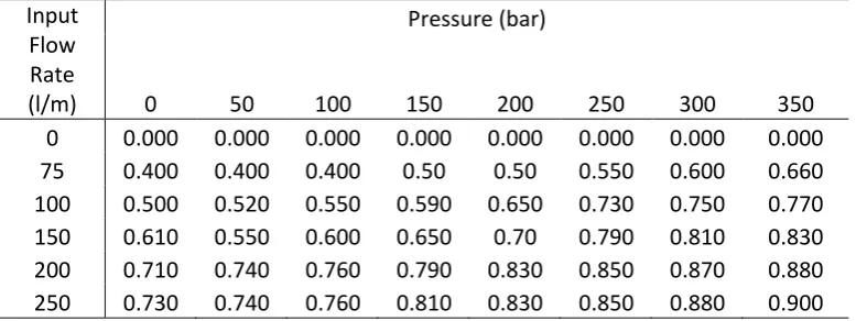
[image:8.595.105.494.585.731.2]Hydraulic pump: The maximum pressure is 350 bar, the maximum flow rate is 250 litres/minute and the data table describing its efficiency curve is given in Table 2.
Input Flow Rate (l/m)
Pressure (bar)
0 50 100 150 200 250 300 350
0 0.000 0.000 0.000 0.000 0.000 0.000 0.000 0.000 75 0.400 0.400 0.400 0.50 0.50 0.550 0.600 0.660 100 0.500 0.520 0.550 0.590 0.650 0.730 0.750 0.770 150 0.610 0.550 0.600 0.650 0.70 0.790 0.810 0.830 200 0.710 0.740 0.760 0.790 0.830 0.850 0.870 0.880 250 0.730 0.740 0.760 0.810 0.830 0.850 0.880 0.900
Hydraulic motor: The maximum pressure is 350 bar, maximum speed is 400 RPM, displacement is 0.628 litres, specific torque is 10Nm/bar, the data table describing the volumetric efficiency curve is given in Table 3, the data table describing the pressure loss curve is given in Table 4 and mechanical efficiency is 0.97.
Pressure (bar) Speed
(RPM) 0 50 100 150 200 250 300 350
0 0.950 0.950 0.950 0.950 0.940 0.930 0.920 0.900 50 0.950 0.950 0.950 0.950 0.940 0.930 0.920 0.900 100 0.950 0.950 0.950 0.960 0.960 0.960 0.950 0.930 150 0.950 0.950 0.950 0.960 0.960 0.960 0.950 0.940 200 0.950 0.950 0.950 0.960 0.960 0.960 0.950 0.950 250 0.950 0.950 0.950 0.950 0.950 0.950 0.950 0.950 300 0.950 0.950 0.950 0.940 0.940 0.940 0.940 0.940 350 0.940 0.940 0.940 0.940 0.940 0.940 0.940 0.940 400 0.940 0.940 0.940 0.940 0.940 0.940 0.940 0.940
Table 3. Hydraulic motor volumetric efficiency data table.
Speed (RPM) 0 50 100 150 200 250 300 350 400 Pressure
loss (bar) 0 1 2 3 5 7 10 14 20
Table 4. Hydraulic motor internal pressure loss data table.
System configuration: Two hydraulic motors and three power units, where each power unit contains a single electric motor and hydraulic pump.
5.2 Component Reliability Models
Electric motor: Accelerated life model with a baseline Weibull time (hours) to failure distribution with scale and shape parameters of 90000 and 1.1 respectively and a data table that describes its covariate curve given by Table 5. The time to install and uninstall from the power unit is 3 hours.
Power
Output (KW) 0 40 80 120 160 Acceleration
factor 0 0.60 0.80 1.00 1.40
Table 5. Electric motor covariate data table.
respectively and a data table that describes its covariate curve given by Table 6. The time to connect and disconnect the hydraulic pump from the hydraulic circuit is 2 hours, whilst the time to install and uninstall from the power unit is 2 hours.
Pressure (bar) Flow
Rate
(l/m) 0 50 100 150 200 250 300 350
0 0 0 0 0 0 0 0 0
[image:10.595.137.460.141.288.2]50 0 0.40 0.40 0.50 0.50 0.55 0.60 0.70 100 0 0.50 0.55 0.55 0.60 0.75 0.80 0.90 150 0 0.55 0.60 0.65 0.85 0.90 1.00 1.10 200 0 0.60 0.65 0.70 0.90 1.10 1.20 1.30 250 0 0.65 0.70 0.75 1.10 1.3 1.50 1.60
Table 6. Hydraulic pump covariate data table.
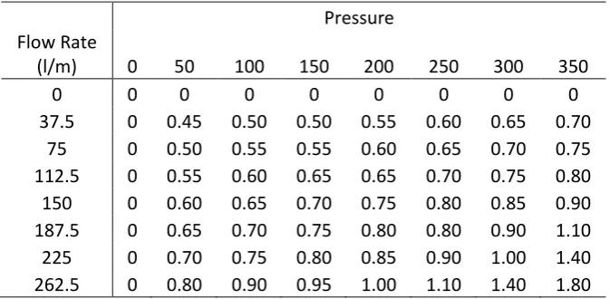
Hydraulic motor: Accelerated life model with a baseline Weibull time (hours) to failure distribution with scale and shape parameters of 68000 and 1.4 respectively and a data table that describes its covariate curve given by Table 7. The time to connect and disconnect the hydraulic motor from the hydraulic circuit is 1 hour, whilst the time to connect and disconnect from the drive shaft is 7 hours.
Pressure Flow Rate
(l/m) 0 50 100 150 200 250 300 350
0 0 0 0 0 0 0 0 0
37.5 0 0.45 0.50 0.50 0.55 0.60 0.65 0.70 75 0 0.50 0.55 0.55 0.60 0.65 0.70 0.75 112.5 0 0.55 0.60 0.65 0.65 0.70 0.75 0.80 150 0 0.60 0.65 0.70 0.75 0.80 0.85 0.90 187.5 0 0.65 0.70 0.75 0.80 0.80 0.90 1.10 225 0 0.70 0.75 0.80 0.85 0.90 1.00 1.40 262.5 0 0.80 0.90 0.95 1.00 1.10 1.40 1.80
Table 7. Hydraulic motor covariate data table.
5.3 Functional Operating Profile Models
Two functional operating profiles are used, named A and B, where profile B has higher average power output and is therefore expected to be more stressful on the drive system.
[image:10.595.130.467.425.590.2]Profile B: 8 hours at 240 RPM speed and 6200 Nm torque, then 16 hours at 360 RPM speed and 6200 Nm torque, repeated in 24 hour cycles.
6. Availability and Maintenance Requirement Results for Example Drive System
1000 tests were performed on the hydraulic system under each of the functional operating profiles, where each test consisted of a simulated 10 year operating period. The total time taken to compute all 2000 tests was less than 5 minutes on a standard PC with 2.2 GHz CPU and 4GB RAM. Under functional profile A, the mean availability was 0.99954, equal to a mean of 40.3 hours downtime over the 10 operating years in each test. A histogram of the availability in each test under this profile is shown in Figure 2. Under functional profile B, the mean availability was 0.99900, equal to a mean of 87.6 hours downtime over the 10 operating years in each test – more than twice the value under functional profile B. A histogram of the availability in each test under this profile is shown in Figure 3. In profile A, the mean number of electric motor, hydraulic pump and hydraulic motor failures were 1.2, 3.4 and 1.4 respectively whilst in profile B the respective values were 2.5, 7.4 and 3.4.
Figure 2. Histogram of availability in tests for functional profile A.
The distribution of results between different tests under the same functional operating profile as shown in the histograms also demonstrate the value of simulation compared to physical tests where only a few, possibly misleading outlier, data points could be produced despite requiring far greater time and financial resources.
7. Conclusions
The availability and maintenance support requirements for a hydraulic drive system operating in a particular application are of importance to manufacturers and customers as downtime and maintenance support are two of the three most significant operating costs, the other being energy usage. A simulation model has been described in this paper that is capable of predicting these values. This was demonstrated through the results shown for an example hydraulic drive system that was analysed operating in two different functional operating profiles using the simulation model. The model is valuable to manufacturers for optimising hydraulic system designs and planning support requirements for particular customer applications. This is of increasing importance due to the growth of the functional product (FP) business model. Analysing a system with the model requires negligible time and financial resources and produces statistics of high practical value.
8. Future Work
Two potential avenues for future work are given below:
Energy consumption analysis: The simulation model presented in this paper predicts the availability and maintenance requirements of a hydraulic drive system operating under a particular functional profile. However, energy usage is also a significant contributor to the operating costs of a hydraulic drive. The model already incorporates detailed efficiency models for each of the hydraulic system components in order to correctly determine system operating parameters that influence reliability. It could therefore also be used to obtain the energy efficiency and consumption of a complete hydraulic drive system under a particular functional profile.
Optimised system configuration and component dimensioning: The development of an algorithm to automatically choose the specifications and number of electric motors, hydraulic pumps and hydraulic motor components that gives optimised performance when given an operating profile and set of available component specifications to choose from by the user. Automating this process has the potential to save a considerable amount of time and money for both hydraulic drive manufacturers and their customers.
Acknowledgments
References
1. Nelson W.B., Accelerated Testing, 2nd Revised Edition, Wiley-Blackwell, (2004).
2. Karlsson M., Lindström J., Löfstrand M., Functional Products – Goodbye to the industrial age, Ericsson Business Review, Volume 18, Issue 2, pp 21-24, (2012).
3. Andrews, J.D., Moss, T.R., Reliability and Risk Assessment, 2nd Edition, Wiley-Blackwell, (2002).
4. Meeker O.M., Escobar L.A., Statistical Methods for Reliability Data, Wiley-Interscience, (1998).
5. Marshall A.W., Olkin I., Life Distributions: Structure of Nonparametric, Semiparametric and Parametric Families, Springer, (2007).
6. Sundin E., Bras B., Making functional sales environmentally and economically beneficial through product remanufacturing, Journal of Cleaner Production, Volume 13, Issue 9, pp 913-925, (2005).
7. Löfstrand M., Kyösti P., Reed S., Backe B., Evaluating availability of functional products through simulation, Simulation Modelling Practice and Theory, Volume 47, pp 196-209, (2014).
8. Reed S., Löfstrand M., Karlsson L., Andrews J., Service Support System Modelling Language for Simulation-driven Development of Functional Products, Procedia CIRP, Volume 11, pp 420-424, (2013).
9. Hillbom J., Powerful Engineering, Hägglunds Drives, (1997).
10. Finkelstein, M.S., Wearing-out of components in a variable environment, Reliability Engineering & System Safety, Volume 66, Issue 3, pp 235-242, (1999).
11. Kijima M., Some results for repairable systems with general repair, Journal of Applied Probability, Volume 26, Issue 1, pp 89-102, (1989). 12. Leemis L.M., Park S.K., Discrete-event Simulation: A first course, Pearson
Prentice Hall, (2006).
13. Skeet, J., C# in Depth, Manning Publications, 3rd Edition, (2013).