Edited by:
Valery M. Nakariakov, University of Warwick, United Kingdom
Reviewed by:
Jiajia Liu, University of Sheffield, United Kingdom Sergey Anfinogentov, Institute of Solar-Terrestrial Physics (RAS), Russia
*Correspondence:
David J. Pascoe david.pascoe@kuleuven.be
Specialty section:
This article was submitted to Stellar and Solar Physics, a section of the journal Frontiers in Astronomy and Space Sciences
Received:18 January 2019
Accepted:20 March 2019
Published:12 April 2019
Citation:
Pascoe DJ, Hood AW and Van Doorsselaere T (2019) Coronal Loop Seismology Using Standing Kink Oscillations With a Lookup Table. Front. Astron. Space Sci. 6:22. doi: 10.3389/fspas.2019.00022
Coronal Loop Seismology Using
Standing Kink Oscillations With a
Lookup Table
David J. Pascoe1*, Alan W. Hood2and Tom Van Doorsselaere1
1Department of Mathematics, Centre for Mathematical Plasma Astrophysics, KU Leuven, Leuven, Belgium,2School of
Mathematics and Statistics, University of St Andrews, St Andrews, United Kingdom
The transverse structure of coronal loops plays a key role in the physics but the small transverse scales can be difficult to observe directly. For wider loops the density profile may be estimated by forward modeling of the transverse intensity profile. The transverse density profile may also be estimated seismologically using kink oscillations in coronal loops. The strong damping of kink oscillations is attributed to resonant absorption and the damping profile contains information about the transverse structure of the loop. However, the analytical descriptions for damping by resonant absorption presently only describe the behavior for thin inhomogeneous layers. Previous numerical studies have demonstrated that this thin boundary approximation produces poor estimates of the damping behavior in loops with wider inhomogeneous layers. Both the seismological and forward modeling approaches suggest loops have a range of layer widths and so there is a need for a description of the damping behavior that accurately describes such loops. We perform a parametric study of the damping of standing kink oscillations by resonant absorption for a wide range of inhomogeneous layer widths and density contrast ratios, with a focus on the values most relevant to observational cases. We describe the damping profile produced by our numerical simulations without prior assumption of its shape and compile our results into a lookup table which may be used to produce accurate seismological estimates for kink oscillation observations.
Keywords: magnetohydrodynamics (MHD), Sun: corona, Sun: magnetic fields, Sun: oscillations, waves and instabilities
1. INTRODUCTION
lower density plasma is smooth. Inside this inhomogeneous layer, wave energy is transferred from kink to Alfvén modes where the local Alfvén speed matches the kink speedCk. The timescale of this process is comparable to the period of oscillation (e.g., Hollweg and Yang, 1988; Goossens et al., 1992, 2002; Ruderman and Roberts, 2002).
Resonant absorption is a robust mechanism which occurs even in loops which are not cylindrically symmetric (Terradas et al., 2008b; Pascoe et al., 2011). Furthermore, numerical studies demonstrate that the Kelvin-Helmholtz instability (e.g., Terradas et al., 2008a; Antolin et al., 2015; Okamoto et al., 2015; Magyar and Van Doorsselaere, 2016; Hillier et al., 2019) is most efficient in loops with thin inhomogeneous layers. This instability leads to a mixing of plasma and effective widening of the inhomogeneous layer (e.g.,Goddard et al., 2018; Karampelas and Van Doorsselaere, 2018) in addition to increased heating due to phase mixing (e.g., Heyvaerts and Priest, 1983; Karampelas et al., 2017; Pagano et al., 2018; Guo et al., 2019) which can account for observations of broad differential emission measures in coronal loops (Van Doorsselaere et al., 2018).
The transverse density profile can be described by two dimensionless parameters; the density contrast ratio being the ratio of the density at the center of the loop to the density far from itζ = ρ0/ρe, and the width of the inhomogeneous layer normalized to the minor loop radiusǫ =l/R. The damping rate due to resonant absorption depends on both of these parameters. For this reason the problem is underdetermined when trying to infer ζ and ǫ from the (exponential) damping time alone and some additional information is required (e.g., Goossens et al., 2008; Arregui and Asensio Ramos, 2014; Arregui and Goossens, 2019).Pascoe et al. (2013)produced a more accurate description of the damping profile due to resonant absorption, which includes the initial Gaussian damping regime of kink oscillations in addition to the later exponential damping regime. This damping profile is characterized by two damping times and so allows both ζ and ǫ to be estimated. This method was first applied byPascoe et al. (2016)and later extended by Pascoe et al. (2017a,c) to include additional effects such as a time-dependent period of oscillation, the presence of additional parallel harmonics, and the use of Bayesian analysis (e.g., Arregui et al., 2013; Arregui, 2018) to improve the estimation of uncertainties. This seismological method requires both the Gaussian and exponential damping regimes to be accurately detected in the data and so depends on the oscillation data having a sufficiently high quality.
Another method for estimatingǫis by forward modeling the appearance of the density profile for direct comparison with the
thin boundary (TB) approximation. To correct for this effect, Pascoe et al. (2018)performed a narrow parametric study using the TB estimate as a starting point. The result of this study was a change in the estimated value of ζ from the TB value of 2.3 to a value of 2.8 based on numerical simulations for
ǫ = 0.9. This case demonstrates the need for a seismological method that can account for the behavior of kink oscillations in loops with wide inhomogeneous layers without the need for separate studies and corrections applied afterwards. The use of a self-consistent seismological method is particularly important for future development of techniques for data analysis where multiple observational signatures are forward modeled and a systematic error arising from the TB approximation would have a deleterious influence on other observables. For example, the EUV intensity isI ∝ ρ2and so a change in inferred density contrast from 2.3 to 2.8 in the example above corresponds to an intensity change by a factor of approximately 1.5.
In this paper we study the behavior of kink oscillations of coronal loops for various transverse density profiles. Our aim is to provide a simple method of estimating the damping profile for a chosen profile which may be used for seismological investigations. The damping profiles for resonant absorption used in previous studies and this one are described in section 2. The results of our parametric study and the generation of a lookup table (LUT) are presented in section 3. In section 4 we present examples of the application of our method to synthetic test cases and observational data. Conclusions are presented in section 5.
2. DAMPING PROFILE FOR KINK
OSCILLATIONS
Initial applications of resonant absorption to explain the strong damping of kink oscillations (Goossens et al., 1992, 2002; Ruderman and Roberts, 2002) considered only the asymptotic state of the system. The damping profile was an exponential of the form
D(t) = exp
− t
τd
, (1)
τd = 4P
this paper we consider a linear profile for the density in the inhomogeneous layer since it is the simplest smooth profile, can describe the widest range of possible structures, and is the only profile for which the analytical solution for all times is presently known (see discussion section 6.2 ofPascoe et al., 2018).
Numerical simulations byPascoe et al. (2012)demonstrated that the damping profile of strongly damped propagating kink oscillations is more accurately described by a Gaussian damping profile rather than an exponential one. The existence of these two regimes was reconciled by the analytical description derived by Hood et al. (2013) which described the damping profile for all times and demonstrates that Gaussian and exponential profile can be obtained in the limits of small and large time, respectively. The derivation byHood et al.(2013) was performed for propagating kink waves with the damping rate expressed in terms of damping length scales but we may consider the case of standing kink waves with a damping time using the long wavelength limitλ=CkP, giving
D(t) = exp − t
2
2τg2
!
, (3)
τg = 2P
π κǫ1/2. (4) We note that the relationship between damping length scales (propagating waves) and timescales (standing waves) has been demonstrated explicitly for the exponential regime (e.g., comparing the derivations of Goossens et al., 2002; Terradas et al., 2010) but presently not the Gaussian regime. Nonetheless we demonstrate the applicability of this relationship (proposed by Pascoe et al., 2010) by comparison with our numerical simulations. The applicability of this relationship has also previously been demonstrated in numerical simulations by Ruderman and Terradas (2013) and Magyar and Van Doorsselaere (2016).
Pascoe et al. (2013)proposed a general damping profile (GDP) that combined both of these damping regimes into a single approximation. This is described in terms of a switch from the Gaussian damping profile that applies at the start of the oscillation to the exponential profile which applies later.
D(t) = exp
−t2
2τ2 g
t≤ts
Asexp
−t−ts
τd
t>ts
, (5)
ts =
P
κ, (6)
where the switch from the Gaussian to exponential damping regime occurs attsandAs=D(t=ts).
The above damping profiles are also based on the thin tube approximation. In this limit the period of the fundamental standing kink mode is
Pk=2L/Ck (7)
whereLis the loop length, and the kink speed for a low-βplasma (uniform magnetic field) is
Ck=CA0
s
2ζ
ζ+1, (8) where CA0 is the internal Alfvén speed. The thin tube thin boundary (TTTB) approximation for the period of oscillation of kink modes therefore depends onζ but notǫ (Goossens et al., 2008). However, the parametric studies byVan Doorsselaere et al. (2004) and Soler et al. (2014) find that Pk does depend on ǫ outside of the applicability of the TB approximation.
To illustrate the different damping profiles,Figure 1shows the results of our numerical simulations (described in section 3) for three values ofǫwithζ = 2. For this value of density contrast the GDP suggests a switch from the Gaussian to exponential damping regime att = 3P. For kink oscillations in low density
contrast loops such as these, the Gaussian damping profile (blue curves) provides a much better description than the exponential damping profile (red curves), and the general damping profile (green curves) further improves the description for later times. As expected, all three analytical profiles become poorer asǫincreases and the TB approximation becomes less appropriate.
In this paper we wish to characterize the damping behavior of kink oscillations as accurately as possible, and without prior assumption of the form of the damping profile. The plus symbols inFigure 1represent the amplitudes Ai which we use to characterize the oscillation. These amplitudes are defined at every half cycle of the oscillation. The LUT damping profile (dashed lines) is constructed from these amplitudes by spline interpolation. The dashed lines indicate that this method allows us to accurately describe the damping of the kink oscillation, albeit at a cost of requiring more information. The exponential and Gaussian damping profiles can each be characterized by a single parameter, i.e., the damping time τd or τg. The GDP combines both the Gaussian and exponential damping regimes and so is characterized by both these damping times (with the switch time given in terms of these two parameters in Equation 6). For the six cycles indicated in Figure 1 our interpolation method uses 13 parameters, or more generally 2n+
1 parameters for ncycles. On the other hand, this number is still sufficiently small that the results of hundreds of numerical simulations can be compiled into a lookup table of minimal size. For each of the three simulations in Figure 1, and the additional simulations presented in section 3, the amplitudes
FIGURE 1 |Comparison of kink oscillations calculated by numerical simulations (solid lines) with the analytical damping profiles (colored lines). The red, blue, and green lines correspond to the exponential, Gaussian, and general damping profiles, respectively. The plus symbols represent the amplitudes used to characterize the oscillation in our lookup table (LUT). The LUT damping profiles (dashed lines) are constructed from these amplitudes by spline interpolation. Theleft,middle, and
rightpanels show the results forǫ=0.1, 0.5, and 1.0, withζ=2 for all cases.
to return results for arbitrary values of time in order for it to appropriately handle requests from the user or from a fitting routine transparently i.e., without needing to take the details of individual simulations into account.
3. PARAMETRIC STUDY
In this section we study the behavior of kink oscillations in coronal loops for various combinations of ζ and ǫ. Soler et al. (2014) and Van Doorsselaere et al. (2004) performed similar numerical studies investigating the damping time for the exponential regime. These studies demonstrated that the thin boundary approximation produces poor estimates of the damping behavior in loops with wider inhomogeneous layers.
As in Soler et al. (2014), we consider L/R = 100 which
is typical for observations of standing kink oscillations. Weak dependence of the damping on the longitudinal wavenumber
kz has been demonstrated by Van Doorsselaere et al. (2004). Numerical simulations were performed using a Lax-Wendroff code to solve the linear MHD equations in cylindrical coordinates
(r,θ,z)form = 1 symmetry corresponding to kink oscillations
(and the Alfvén waves generated by resonant absorption). The magnetic field is constant and aligned with the z-direction. This code was previously used in Pascoe et al. (2012, 2013, 2015) and Hood et al. (2013) to study the spatial damping of propagating kink waves and here is applied to the case of the temporal damping of standing kink waves by appropriate choice of boundary and initial conditions. The boundary conditions are line-tied to simulate the loop footpoints being fixed in the photosphere, while the boundary in the r-direction is placed sufficiently far away to not affect the results. The fundamental longitudinal harmonic of the standing kink mode is excited by a perturbation to the radial and azimuthal velocities of the form
v(r,θ,z) = (vr,vθ,vz)=(ξrcosθ,ξθsinθ, 0)sin(πz/L), (9)
ξr(r) =
1 r≤R
R2/r2 r>R , (10)
ξθ(r) =
−1 r≤R
R2/r2 r>R . (11)
In the following simulations, the numerical domain coversr =
[0, 10R] andz = [0, 100R], with a resolution of 1, 000×1, 000 grid points. Each of our 300+ simulations took approximately 1 h to run using 80×2.8 GHz processor cores. We study the standing mode by considering the variation in the amplitude of the transverse velocity measured at the loop apexz=L/2.
Figure 2shows the simulations performed in our parametric study which were used to generate the first version of our lookup table. The solid, dashed, and dotted lines correspond to the damping rates shown in the right panel. These damping profiles are based on the TB approximation for the Gaussian damping profile and so will not accurately describe the behavior for large
ǫ but serve as an indication of the range of parameters we are interested in considering with respect to observational studies. The curves demonstrate that we are not equally interested in all regions of theζ-ǫ parameter space. Large amplitude standing kink oscillations are typically observed for fewer than 6 cycles (e.g., Goddard and Nakariakov, 2016) and so we are mainly interested in parameters which produce this level of damping. The dotted, solid, and dashed lines correspond toτg/P = 1, 2, and 5, respectively, and indicate the parameters we expect to be relevant to observations. For large values of bothζ andǫ, kink oscillations would be very strongly damped and hence unlikely to be reliably detected. The shorter time series available would also generally limit the seismological information that could be obtained. Unlikeǫwhich has the defined upper limit of 2, there is no upper limit forζ. However, the damping rate is asymptotic in this limit and so we can consider a reasonable upper limit, which is taken to be 7 in this study but may be extended in the future (e.g., high contrast filament threads considered byArregui et al., 2008). For small values of bothζ and ǫ the oscillations would be weakly damped. Such oscillations are not typically observed, although we are still interested in the behavior for small values ofǫ with regard to checking convergence of our results to the analytical profiles based on the TB approximation.
FIGURE 2 |The black circles denote the 300 numerical simulations that comprise version 1.0 of our LUT. The solid, dashed, and dotted lines correspond to the damping rates shown in the right panel. These damping profiles are based on the TB approximation for the Gaussian damping profile but serve as an indication of the range of parameters we are interested in considering with respect to observational studies.
space using the IDL routine GRIDDATA which can be used to interpolate our simulation results to return the damping profile for an arbitrary value ofζ and ǫ. Additional simulations were performed for testing purposes, including generating synthetic observational data used in section 4. These additional simulations are not included version 1.0 LUT but may be in future applications of the LUT to actual observational data. The use of a LUT and interpolation methods for scattered data allows the method to be improved over time by incorporating additional results as they are obtained. Other examples of a LUT strategy for solar applications include the CHIANTI emission database (Del Zanna et al., 2015) used as part of EUV forward modeling codes such as FOMO(Van Doorsselaere et al., 2016), and the CAISAR code for inversions of solar Ca II spectra (Beck et al., 2015).
The LUT and the corresponding IDL code are available at https://github.com/djpascoe/kinkLUT. The routine requires as input the values of ǫ, ζ, and the normalized times tn = t/P
at which the damping profile is desired. The value of each amplitudeAiis determined by 2D interpolation of the simulation results using the IDL routine GRIDDATA. (In this paper we use the linear method, chosen as the simplest method with fewest assumptions, for which requested grid points are linearly interpolated from triangles formed by Delaunay triangulation. These triangles were constructed with the TRIANGULATE routine and are included in the LUT save file). The damping profile is then returned by spline interpolation of these amplitudesAifor the user-requested timestn. This procedure can be used within a forward modeling function used for comparing a model with data. For example, a simple model for an oscillation with a single harmonic and no background trend, as considered in this paper, is
y(t)=A0sin
2πt
P +φ
DLUT(tn,ǫ,ζ ), (12)
whereA0is the initial amplitude of a sinusoidal oscillation with periodPand phase shiftφ, and the damping profileDLUTis based
on our lookup table. We demonstrate the results of such a method in section 4.
3.1. Dependence of Period of Oscillation
and Damping Rate on Transverse Density
Profile
Here we compare the results of our parametric study with the analytical profiles discussed in section 2 and previous numerical studies.
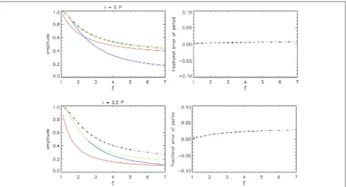
Figure 3shows the dependence of the kink mode behavior on ζ. For an exponential or Gaussian damping profile it is convenient to characterize the damping with the damping time (or length scale for propagating waves). However, in this study we make no assumption about the shape of the damping profile and so we consider the damping which has occurred after a certain time, or a certain number of oscillation cycles since the period of oscillation also depends onζ. The colored lines correspond to the theoretical damping rates based on the TB approximation and an exponential (red), Gaussian (blue), or general (green) damping profile.
The top panels ofFigure 3 demonstrate the case of a thin inhomogeneous layer (ǫ = 0.1) where the TB approximation
is appropriate. The top left panel reproduces the known dependence of the shape of the damping profile on ζ. For lower density contrasts the Gaussian profile better describes the damping. The GDP which combines both profiles, with a switch from Gaussian to exponential that depends on ζ, provides a significantly better approximation for all values ofζ. The switch time occurs at 5Pforζ = 1.5 and so the general and Gaussian damping profiles are identical forζ≤1.5.
The bottom panels ofFigure 3demonstrate the case of a finite inhomogeneous layer (ǫ = 0.5) where the TB approximation is less appropriate. The estimated period of oscillation is still reasonable but the damping is being significantly overestimated. The amplitude is taken at the earlier time of 2.5P since the damping is stronger for the larger value ofǫ. At this earlier time, the Gaussian damping profile is always a better approximation than the exponential profile for the range ofζ ≤ 7 considered. The switch time occurs at 2.5P for ζ ≈ 2.3, and so it is
FIGURE 3 |Dependence of the damping of the kink oscillation on the density contrast ratioζ. Thetoppanels show results forǫ=0.1 and thebottompanels for ǫ=0.5. The left panels show the kink oscillation amplitude (plus symbols) taken at a fixed time (t=5Por 2.5P) The colored lines show the estimates based on the general damping profile (green), Gaussian damping profile (blue), and exponential damping profile (red). The right panels show the variation of the period of oscillation compared with the theoretical valuePk.
so poor during the first cycle or so. The Gaussian estimate therefore does not become poorer than the exponential estimate by the time of 2.5Pconsidered in the bottom panel ofFigure 3, whereas it does in the top panel. Whether the Gaussian or exponential estimate is better therefore depends on not only when the switch occurs but also how much data is considered after that switch. The general damping profile provides the best approximation for all parameters and times, but is also inaccurate when there is significant damping due to the limitations of the TB approximation it is based upon.
The right panels of Figure 3 show the fractional error in the period of oscillation estimated as Pk by Equation (7). The
errors are typically very small since the thin tube approximation (ω/kz=Ck) is appropriate for our simulations withL/R=100. The error increases withζdue to the stronger dispersion present in higher contrast loops, and is also found to increase withǫ(see alsoFigures 4,6).
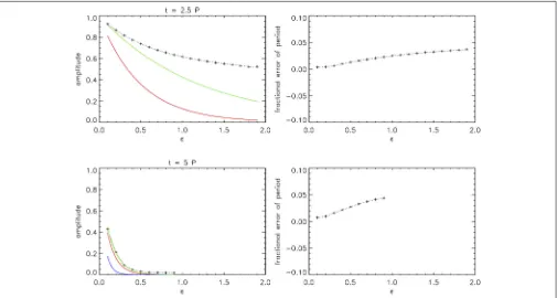
Figure 4shows the dependence of the kink mode behavior on
ǫ. The top panels show results forζ = 2 att = 2.5P, i.e., the behavior at an early time for a low density contrast ratio. For
ζ =2 the switch for Gaussian to exponential occurs att=3Pand so the Gaussian and general damping profiles are identical before this time, and are a significantly better approximation than the exponential profile. The bottom panels show results forζ =7 at t=5P, i.e., having both a sufficiently high density contrast and a sufficiently large number of cycles for the exponential damping
profile to always be a better approximation than the Gaussian profile, though the GDP remains an improvement over both.
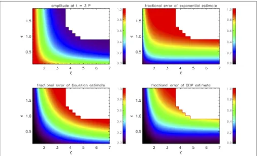
Figure 5shows 2D contours for the amplitude of the kink oscillation att = 3P(top left panel) and the fractional errors of the corresponding estimates based on the TB approximation. The errors tend to zero in the appropriate limitǫ→0, otherwise each approximation underestimates the amplitude. The Gaussian and GDP estimates are also accurate in the limitζ → 1 since they describe the initial stage of resonant absorption, whereas the exponential estimates remain poor in this limit whenǫ >0.
Figure 6shows the fractional error in the period of oscillation estimated using the TB approximation (Equation 7). The TB approximation underestimates the period of oscillation. The dependence of the error on ζ and ǫ is similar to that found bySoler et al. (2014) (i.e., being proportional to the strength of the damping due to resonant absorption) but the magnitude is smaller, remaining less than 6%.Soler et al. (2014)report an error of up to 45% in their study which considersζ up to 20, whereas we restrict our attention to the parameter range most relevant to observations (e.g.,ζ ≤3.5 for the largest values ofǫ
inFigure 2). However, even accounting for this there remains a discrepancy andSoler et al. (2014)find errors greater than 30% for a comparable parameter range.
FIGURE 4 |Dependence of the damping of the kink oscillation on the inhomogeneous layer widthǫ. Thetoppanels show results forζ=2 and thebottompanels forζ=7. The left panels show the kink oscillation amplitude (plus symbols) taken at a fixed time (t=5Por 2.5P) The colored lines show the estimates based on the general damping profile (green), Gaussian damping profile (blue), and exponential damping profile (red). The right panels show the variation of the period of oscillation compared with the theoretical valuePk.
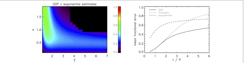
improvement over the exponential profile, and the difference is largest for lowerζ, typically∼ 60% forζ < 2 and∼ 30% for
ζ >2. The right panel ofFigure 7shows how the fractional error (averaged over 300 numerical simulations) varies as a function of time for each of the profiles based on the TB approximation. Each of the errors increase in time due to the cumulative effect of overestimating the damping rate, however the GDP remains at all times a significantly better estimate of the kink oscillation amplitude. The GDP (Equation 6) is a simple modification of the exponential damping profile with no additional parameters and so this improved estimate comes at effectively no computational cost. Our LUT method is based on several interpolation routines and so is slower to calculate than the GDP but remains practical. The larger errors for analysis based on the exponential profile arise because it provides a very poor description for the initial behavior of kink oscillations. Pascoe et al. (2013) demonstrate that the seismological estimate based on the exponential profile is significantly improved by ignoring the first two cycles of the oscillation and only analysing the remaining data. However, this is not a practical solution for detailed analysis of oscillations since it means the initial amplitude cannot be estimated, which is important for nonlinear effects. It would also hinder the potential to detect higher harmonic oscillations which have a shorter period and so typically only exist for the first few cycles of the fundamental mode (e.g.,Pascoe et al., 2017a). For example, if the fundamental mode is observable for six cycles then the third harmonic with P3 ≈ P1/3 but the same damping per
period would only be detectable during the first two cycles of the fundamental mode.
4. SEISMOLOGICAL APPLICATION
In this section we demonstrate the application of our LUT as a seismological tool to use the observed damping of a kink oscillation to infer information about the transverse density profile of the oscillating loop.
Figure 8shows the results of a test of our method for a kink oscillation simulated in a loop withζ = 2.15 andǫ = 0.75. This data point is not included in version 1.0 of our LUT used in the following analysis. The top panel shows the analyzed oscillation which includes uniformly distributed random noise with a maximum amplitude of 5% of the initial kink oscillation amplitude. The middle and bottom panels show 2D histograms approximating the marginalized posterior probability density function forζ andǫ based on 105 Markov chain Monte Carlo (MCMC) samples of the GDP and LUT models, respectively (see also Pascoe et al., 2017a, 2018). This data comes from a simulation with an inhomogeneous layer width that is sufficiently large for the TB approximation to produce inaccurate results. The GDP approach overestimates the value ofǫ, and correspondingly underestimates the value ofζ.
FIGURE 5 |Amplitude of the kink oscillation att=3P(top left)and the fractional errors of the corresponding estimates based on the TB approximation and an exponential(top right), Gaussian(bottom left), or the general(bottom right)damping profiles.
FIGURE 6 |Error in the period of oscillation estimate based on the TB approximation as given by Equation (7).
and ǫ, aside from the quality of the observational data. Due to the asymptotic nature of the inversion curve, the extent to whichζ andǫare constrained depends on whether the density contrast is high or low; near the low-ζ asymptote ζ is well-constrained but ǫ is poorly constrained, and vice versa for the high-ζ asymptote. This is demonstrated in Figure 8where the
GDP inversion underestimates the actual value ofζ = 2.15 and produces very low estimates ofζ. The red bars indicate the 95% credible intervals and show the value ofζis well-constrained (but excludes the actual value ofζ due to the systematic error from the TB approximation). In comparison, the inversion results using the LUT are less constrained forζ but the maximum a posteriori probability (MAP) estimate ofζ ≈ 2.11 is consistent with the actual value for the synthetic data. The nature of these constraints makes 2D histograms such as those inFigure 9the simplest way of representing the available information for the transverse density profile. Quoting confidence intervals alone can be misleading if the asymptotic behavior is not kept in mind. Furthermore, 1D histograms forζ and ǫ would generally not be well described using a normal distribution (they have been approximated by the exponentially modified Gaussian function byPascoe et al., 2017a) and so estimates of uncertainties based on assuming this distribution would not be accurate.
FIGURE 7 |Difference between the fractional error using the exponential damping profile alone compared with the GDP(left), and the mean fractional error as a function of time for each of the three TB profiles(right).
4.1. Comparison With Previous
Spatiotemporal Analysis
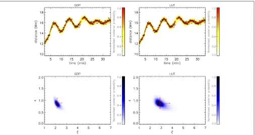
Pascoe et al. (2018) presented a method for spatiotemporal analysis of coronal loops which used both the transverse EUV intensity profile and the standing kink oscillation to constrain the properties of the coronal loop. In that work the spatial analysis (forward modeling of the transverse EUV profile) provided a value of ǫ ≈ 0.9 and so a narrow parametric study for that particular observation was performed to estimate the effect of a thick inhomogeneous layer on the seismological component of their analysis. Here we demonstrate how the results may be reproduced from the much wider parametric study in this paper. Figure 10 shows the results of applying our method to the oscillation of Leg 1 as previously analyzed. We consider the prior for ǫ with the form of a normal distribution with a mean of 0.9 and standard deviation of 0.1 (e.g., Figure 4 of Pascoe et al., 2018). The seismological analysis of the oscillation then proceeds as in section 4.1 of Pascoe et al. (2018), with results based on 106 MCMC samples of a model consisting of a damped sinusoidal oscillation which begins at a start time
t0 ≈ 4 minutes and having a background trend described by spline interpolation using six reference points across the time series. We consider both the GDP and LUT damping profiles. The top panels inFigure 10show the loop position (plus symbols) with the color contour representing the normalized posterior predictive probability density for each damping profile model. The GDP (left panels) results infer a value ofζ =2.1+0.4
−0.2(based on the MAP value and 95% credible interval) consistent with the previous analysis. The narrow parametric study in section 6.4 of Pascoe et al. (2018)suggestedζ ≈2.8 as an improved estimate, correcting for the TB approximation used in the GDP. The right panels ofFigure 10show our analysis using the LUT damping profile, which infersζ = 2.9+0.9
−0.5, consistent with that estimate. The Bayes factor (e.g.,Jeffreys, 1961; Kass and Raftery, 1995) for the LUT model compared with the GDP isK=1.5, i.e., too small to distinguish which model is better based on their reproduction of the data alone. This is in contrast to the very strong Bayesian evidence for the GDP compared with an exponential damping profile found in Pascoe et al. (2018). For this data, the shape of the damping profile produced by the LUT is very similar to
the shape produced by the GDP (but significantly different to an exponential damping profile), though the inferred values of
ζ andǫ that correspond to that shape differ. Considering that
ǫ≈0.9 whereas the GDP is based on the TB approximation, the LUT method is more appropriate on the basis of self-consistency. The GDP underestimates the LUT density contrast ratio by approximately 25%, and analysis using an exponential damping profile underestimatesζby approximately 50%.
The observation considered byPascoe et al. (2018)was one for which the spatial analysis provided a well-constrained value ofǫ, independent of the seismological analysis. It was therefore possible in that study to consider the correction to the TB approximation in terms of the dependence onζ alone, requiring only a narrow 1D parametric study for the estimate. The LUT for the 2D parametric study in this paper allows the method in Pascoe et al. (2018)to be extended to a greater number of loops where the spatial information might not be as conclusive on its own but can assist in further constraining the seismologically-inferred parameters.
5. CONCLUSIONS
In this paper we have performed a parametric study for the dependence of the damping of standing kink oscillations by resonant absorption on the density contrast ratio ζ and the width of the inhomogeneous layer ǫ. Previous studies (Van Doorsselaere et al., 2004; Soler et al., 2014) have demonstrated the inaccuracy of the classical analytical description for the damping rateτd, which is based on the TB approximation, when applied to loops with large values of ǫ. We have expanded on these studies by developing a description of the damping profile which includes the initial non-exponential regime, and summarized our results into a lookup table which may be used to produce improved estimates of loop parameters.
FIGURE 8 |Thetoppanel shows a test kink oscillation simulated forζ=2.15
andǫ=0.75 with noise added. Themiddleandbottompanels show the seismologically estimated transverse density structure based on the GDP and LUT methods, respectively. The color contours represent the normalized 2D histograms approximating the marginalized posterior probability density function. The red error bars correspond to the MAP value and 95% credible intervals, and the green circle indicates the actual density profile parameters.
effects which depend on the density profile parameters. On the other hand, this work only accounts for the influence of wide inhomogeneous layers on the kink oscillation damping profile, with other assumptions and approximations needing to be considered.
FIGURE 9 |Seismological test as inFigure 8forζ=3.75 andǫ=0.2.
FIGURE 10 |Analysis of the oscillation reported inPascoe et al. (2018)using the GDP and LUT damping profile. Thetoppanels show the position of Leg 1 (plus symbols) with the color contour representing the normalized posterior predictive probability density for each damping model.Bottompanels as inFigure 8.
and that choosing a different profile would return a different answer. However, presently no such choice exists since the linear profile is the only one for which a full analytical solution is known (Hood et al., 2013; Ruderman and Terradas, 2013). The linear profile is therefore the natural choice of profile for use in this study, to allow a comparison of numerical results with the TB approximations in the limit ǫ → 0. Pascoe et al. (2018) estimate that the difference in the seismological results using the linear and sinusoidal density profiles is . 10%. However, these two profiles are not the only possible choices. If some profile (other than the linear one used) should be shown to be more appropriate for coronal loops then it would be simple (though computationally expensive) to reproduce our parametric study for that profile. If the spatial resolution of loops is sufficiently high then it is possible to test different profiles by forward modeling the EUV profile (e.g.,Aschwanden et al., 2007; Goddard et al., 2017; Pascoe et al., 2017b, 2018). Such methods still typically involve further assumptions or approximations (e.g., loops having a cylindrical cross-section and azimuthal symmetry) however the aim of these investigations should not be considered the impossible task of inferring the precise density profile of coronal loops but rather estimating the most appropriate characteristic scales that influence the relevant physical processes. Resonant absorption, phase mixing, and the Kelvin-Helmholtz instability all depend on the transverse loop structure. In this context it is not required that the coronal loop density profile is exactly linear for the analysis based on this profile (or any other simplified model) to provide accurate and
useful estimates of parameters such as the size of the transverse inhomogeneityl=ǫR.
Our LUT is also based on results of numerical simulations for the linear regime and so excludes the effect of the Kelvin-Helmholtz instability (KHI). The current technique is therefore more suitable for loops with wider inhomogeneous layers in which KHI develops at a slower rate. Simulations byMagyar and Van Doorsselaere (2016) suggest KHI is weak for ǫ &
of oscillation (and ratios of periods for different longitudinal harmonics) can also be affected by longitudinal structuring due to gravity (e.g., Andries et al., 2005). Cooling of coronal loops causes the scale height to vary in time, accompanied by decreases in the period and period ratio (Morton and Erdélyi, 2009) and an amplification of kink oscillation which acts against the damping due to resonant absorption (Ruderman, 2011). Numerical simulations suggest this effect is typically small but could be approximately 10% for larger amplitude oscillations (Magyar et al., 2015). Similarly, the period of oscillation and period ratio can be affected by expansion of the loop at the apex (Verth and Erdélyi, 2008) and a time-dependent expansion can also reduce the damping of kink oscillations (Shukhobodskiy
DP and TVD contributed conception and design of the study. AH and DP developed the code for the numerical simulations. DP wrote the first draft of the manuscript, and received input from all co-authors.
FUNDING
AH acknowledges funding from the Science and Technology Facilities Council (UK) through the consolidated grant ST/N000609. DP and TVD were supported by the GOA-2015-014 (KU Leuven) and the European Research Council (ERC) under the European Union’s Horizon 2020 research and innovation programme (grant agreement No. 724326).
REFERENCES
Andries, J., Arregui, I., and Goossens, M. (2005). Determination of the coronal density stratification from the observation of harmonic coronal loop oscillations.Astrophys. J. Lett.624, L57–L60. doi: 10.1086/430347
Antolin, P., De Moortel, I., Van Doorsselaere, T., and Yokoyama, T. (2017). Observational signatures of transverse magnetohydrodynamic waves and associated dynamic instabilities in coronal flux tubes.Astrophys. J.836:219. doi: 10.3847/1538-4357/aa5eb2
Antolin, P., Okamoto, T. J., De Pontieu, B., Uitenbroek, H., Van Doorsselaere, T., and Yokoyama, T. (2015). Resonant absorption of transverse oscillations and associated heating in a solar prominence. II. Numerical aspects.Astrophys. J.
809:72. doi: 10.1088/0004-637X/809/1/72
Arregui, I. (2018). Bayesian coronal seismology.Adv. Space Res.61, 655–672. doi: 10.1016/j.asr.2017.09.031
Arregui, I., and Asensio Ramos, A. (2014). Determination of the cross-field density structuring in coronal waveguides using the damping of transverse waves.
Astron. Astrophys.565:A78. doi: 10.1051/0004-6361/201423536
Arregui, I., Asensio Ramos, A., and Pascoe, D. J. (2013). Determination of transverse density structuring from propagating magnetohydrodynamic
waves in the solar atmosphere. Astrophys. J. Lett. 769:L34.
doi: 10.1088/2041-8205/769/2/L34
Arregui, I., and Goossens, M. (2019). No unique solution to the seismological problem of standing kink MHD waves. Astron. Astrophys. 622, 1–10. doi: 10.1051/0004-6361/201833813
Arregui, I., Terradas, J., Oliver, R., and Ballester, J. L. (2008). Damping of fast magnetohydrodynamic oscillations in quiescent filament threads.Astrophys. J. Lett.682:L141. doi: 10.1086/591081
Aschwanden, M. J., de Pontieu, B., Schrijver, C. J., and Title, A. M. (2002). Transverse oscillations in coronal loops observed with TRACE II. Measurements of geometric and physical parameters.Solar Phys.206, 99–132. doi: 10.1023/A:1014916701283
Aschwanden, M. J., Fletcher, L., Schrijver, C. J., and Alexander, D. (1999). Coronal loop oscillations observed with the transition region and coronal explorer.
Astrophys. J.520, 880–894. doi: 10.1086/307502
Aschwanden, M. J., Nightingale, R. W., and Boerner, P. (2007). A statistical model of the inhomogeneous corona constrained by triple-filter measurements
of elementary loop strands with TRACE. Astrophys. J. 656, 577–597. doi: 10.1086/510232
Beck, C., Choudhary, D. P., Rezaei, R., and Louis, R. E. (2015). Fast inversion of solar ca ii spectra.Astrophys. J.798:100. doi: 10.1088/0004-637X/798/2/100 Chen, L., and Hasegawa, A. (1974). Plasma heating by spatial resonance of Alfven
wave.Phys. Fluids17, 1399–1403. doi: 10.1063/1.1694904
De Moortel, I., and Nakariakov, V. M. (2012). Magnetohydrodynamic waves and coronal seismology: an overview of recent results.R. Soc. Lond. Philos. Trans. Ser. A370, 3193–3216. doi: 10.1098/rsta.2011.0640
De Moortel, I., Pascoe, D. J., Wright, A. N., and Hood, A. W. (2016). Transverse, propagating velocity perturbations in solar coronal loops.Plasma Phys. Control. Fus.58:014001. doi: 10.1088/0741-3335/58/1/014001
Del Zanna, G., Dere, K. P., Young, P. R., Landi, E., and Mason, H. E. (2015). CHIANTI - An atomic database for emission lines. Version 8. Astron.
Astrophys.582:A56. doi: 10.1051/0004-6361/201526827
Goddard, C. R., Antolin, P., and Pascoe, D. J. (2018). Evolution of the transverse density structure of oscillating coronal loops inferred by forward modeling of EUV intensity.Astrophys. J.863:167. doi: 10.3847/1538-4357/ aad3cc
Goddard, C. R., and Nakariakov, V. M. (2016). Dependence of kink oscillation damping on the amplitude. Astron. Astrophys. 590:L5. doi: 10.1051/0004-6361/201628718
Goddard, C. R., Nisticò, G., Nakariakov, V. M., and Zimovets, I. V. (2016). A statistical study of decaying kink oscillations detected using SDO/AIA.Astron.
Astrophys.585:A137. doi: 10.1051/0004-6361/201527341
Goddard, C. R., Pascoe, D. J., Anfinogentov, S., and Nakariakov, V. M. (2017). A statistical study of the inferred transverse density profile of coronal loop threads observed with SDO/AIA.Astron. Astrophys.605:A65. doi: 10.1051/0004-6361/201731023
Goossens, M., Andries, J., and Aschwanden, M. J. (2002). Coronal loop oscillations. An interpretation in terms of resonant absorption of quasi-mode kink oscillations. Astron. Astrophys. 394, L39–L42. doi: 10.1051/0004-6361:200 21378
Goossens, M., Hollweg, J. V., and Sakurai, T. (1992). Resonant behaviour of MHD waves on magnetic flux tubes. III - Effect of equilibrium flow.Solar Phys.138, 233–255. doi: 10.1007/BF00151914
Guo, M., Van Doorsselaere, T., Karampelas, K., Li, B., Antolin, P., and De Moortel, I. (2019). Heating effects from driven transverse and Alfvén waves in coronal loops.Astrophys. J.870. doi: 10.3847/1538-4357/aaf1d0
Heyvaerts, J., and Priest, E. R. (1983). Coronal heating by phase-mixed shear Alfven waves.Astron. Astrophys.117, 220–234.
Hillier, A., Barker, A., Arregui, I., and Latter, H. (2019). On Kelvin-Helmholtz and parametric instabilities driven by coronal waves.Month. Notices R. Astron. Soc.
482, 1143–1153. doi: 10.1093/mnras/sty2742
Hollweg, J. V., and Yang, G. (1988). Resonance absorption of compressible magnetohydrodynamic waves at thin ’surfaces’.JGR Space Phys.93, 5423–5436. Hood, A. W., Ruderman, M., Pascoe, D. J., De Moortel, I., Terradas, J., and Wright, A. N. (2013). Damping of kink waves by mode coupling. I. Analytical treatment.
Astron. Astrophys.551:A39. doi: 10.1051/0004-6361/201220617
Jeffreys, H. (1961).Theory of Probability. 3rd Edition. Oxford:Clarendon Press.
Karampelas, K., and Van Doorsselaere, T. (2018). Simulations of
fully deformed oscillating flux tubes. Astron. Astrophys. 610:L9. doi: 10.1051/0004-6361/201731646
Karampelas, K., Van Doorsselaere, T., and Antolin, P. (2017). Heating by transverse waves in simulated coronal loops. Astron. Astrophys.604:A130. doi: 10.1051/0004-6361/201730598
Kass, R. E., and Raftery, A. E. (1995). Bayes factors.J. Am. Stat. Assoc.90, 773–795. doi: 10.1080/01621459.1995.10476572
Lemen, J. R., Title, A. M., Akin, D. J., Boerner, P. F., Chou, C., Drake, J. F., et al. (2012). The Atmospheric Imaging Assembly (AIA) on the Solar Dynamics Observatory (SDO).Solar Phys.275, 17–40. doi: 10.1007/s11207-011-9776-8 Magyar, N., and Van Doorsselaere, T. (2016). Damping of nonlinear standing kink
oscillations: a numerical study.Astron. Astrophys.595:A81. doi: 10.1051/0004-6361/201629010
Magyar, N., Van Doorsselaere, T., and Marcu, A. (2015). Numerical simulations of transverse oscillations in radiatively cooling coronal loops.Astron. Astrophys.
582:A117. doi: 10.1051/0004-6361/201526287
Markwardt, C. B. (2009). “Non-linear Least-squares Fitting in IDL with MPFIT,” in
Astronomical Data Analysis Software and Systems XVIII, Vol. 411, Astronomical Society of the Pacific Conference Series, eds D. A. Bohlender, D. Durand, and P. Dowler (San Francisco, CA), 251.
Morton, R. J., and Erdélyi, R. (2009). Transverse oscillations of a cooling coronal loop.Astrophys. J.707, 750–760. doi: 10.1088/0004-637X/707/1/750 Nakariakov, V. M., and Ofman, L. (2001). Determination of the coronal
magnetic field by coronal loop oscillations.Astron. Astrophys.372, L53–L56. doi: 10.1051/0004-6361:20010607
Nakariakov, V. M., Ofman, L., Deluca, E. E., Roberts, B., and Davila, J. M. (1999). TRACE observation of damped coronal loop oscillations: Implications for coronal heating. Science 285, 862–864. doi: 10.1126/science.285. 5429.862
Nisticò, G., Nakariakov, V. M., and Verwichte, E. (2013). Decaying and decayless transverse oscillations of a coronal loop.Astron. Astrophys.552:A57. doi: 10.1051/0004-6361/201220676
Okamoto, T. J., Antolin, P., De Pontieu, B., Uitenbroek, H., Van Doorsselaere, T., and Yokoyama, T. (2015). Resonant absorption of transverse oscillations and associated heating in a solar prominence. I. Observational aspects.Astrophys. J.
809:71. doi: 10.1088/0004-637X/809/1/71
Pagano, P., Pascoe, D. J., and De Moortel, I. (2018). Contribution of phase-mixing of Alfvén waves to coronal heating in multi-harmonic loop oscillations.Astron.
Astrophys.616:A125. doi: 10.1051/0004-6361/201732251
Pascoe, D. J. (2014). Numerical simulations for MHD coronal seismology.Res.
Astron. Astrophys.14, 805–830. doi: 10.1088/1674-4527/14/7/004
Pascoe, D. J., Anfinogentov, S., Nisticò, G., Goddard, C. R., and Nakariakov, V. M. (2017a). Coronal loop seismology using damping of standing kink oscillations by mode coupling. II. additional physical effects and Bayesian analysis.Astron.
Astrophys.600:A78. doi: 10.1051/0004-6361/201629702
Pascoe, D. J., Anfinogentov, S. A., Goddard, C. R., and Nakariakov, V. M. (2018). Spatiotemporal analysis of coronal loops using seismology of damped kink oscillations and forward modeling of EUV intensity profiles.Astrophys. J.
860:31. doi: 10.3847/1538-4357/aac2bc
Pascoe, D. J., Goddard, C. R., Anfinogentov, S., and Nakariakov, V. M. (2017b). Coronal loop density profile estimated by forward modelling of EUV intensity.
Astron. Astrophys.600:L7. doi: 10.1051/0004-6361/201730458
Pascoe, D. J., Goddard, C. R., Nisticò, G., Anfinogentov, S., and Nakariakov, V. M. (2016). Coronal loop seismology using damping of standing kink oscillations by mode coupling. Astron. Astrophys. 589:A136. doi: 10.1051/0004-6361/201628255
Pascoe, D. J., Hood, A. W., de Moortel, I., and Wright, A. N. (2012). Spatial damping of propagating kink waves due to mode coupling.Astron. Astrophys.
539:A37. doi: 10.1051/0004-6361/201117979
Pascoe, D. J., Hood, A. W., De Moortel, I., and Wright, A. N. (2013). Damping of kink waves by mode coupling. II. Parametric study and seismology.Astron.
Astrophys.551:A40. doi: 10.1051/0004-6361/201220620
Pascoe, D. J., Russell, A. J. B., Anfinogentov, S. A., Simões, P. J. A., Goddard, C. R., Nakariakov, V. M., et al. (2017c). Seismology of contracting and expanding coronal loops using damping of kink oscillations by mode coupling.Astron.
Astrophys.607:A8. doi: 10.1051/0004-6361/201730915
Pascoe, D. J., Wright, A. N., and De Moortel, I. (2010). Coupled Alfvén and Kink Oscillations in Coronal Loops. Astrophys. J. 711, 990–996. doi: 10.1088/0004-637X/711/2/990
Pascoe, D. J., Wright, A. N., and De Moortel, I. (2011). Propagating coupled Alfvén and kink oscillations in an arbitrary inhomogeneous corona.Astrophys. J.
731:73. doi: 10.1088/0004-637X/731/1/73
Pascoe, D. J., Wright, A. N., De Moortel, I., and Hood, A. W. (2015). Excitation and damping of broadband kink waves in the solar corona.Astron. Astrophys.
578:A99. doi: 10.1051/0004-6361/201321328
Roberts, B. (2008). “Progress in coronal seismology,” inIAU Symposium, Vol. 247, eds R. Erdélyi and C. A. Mendoza-Briceno (Cambridge), 3–19.
Ruderman, M. S. (2011). Resonant damping of kink oscillations
of cooling coronal magnetic loops. Astron. Astrophys. 534:A78.
doi: 10.1051/0004-6361/201117416
Ruderman, M. S., and Roberts, B. (2002). The damping of coronal loop oscillations.
Astrophys. J.577, 475–486. doi: 10.1086/342130
Ruderman, M. S., and Terradas, J. (2013). Damping of coronal loop kink oscillations due to mode conversion. Astron. Astrophys. 555:A27. doi: 10.1051/0004-6361/201220195
Russell, A. J. B., Simões, P. J. A., and Fletcher, L. (2015). A unified view of coronal loop contraction and oscillation in flares.Astron. Astrophys.581:A8. doi: 10.1051/0004-6361/201525746
Sarkar, S., Pant, V., Srivastava, A. K., and Banerjee, D. (2016). Transverse oscillations in a coronal loop triggered by a jet.Solar Phys.291, 3269–3288. doi: 10.1007/s11207-016-1019-6
Shukhobodskiy, A. A., Ruderman, M. S., and Erdélyi, R. (2018). Resonant damping of kink oscillations of thin cooling and expanding coronal magnetic loops.Astron. Astrophys. 619:A173. doi: 10.1051/0004-6361/2018 33714
Soler, R., Goossens, M., Terradas, J., and Oliver, R. (2014). The behavior of transverse waves in nonuniform solar flux tubes. II. Implications for coronal loop seismology.Astrophys. J.781:111. doi: 10.1088/0004-637X/781/ 2/111
Stepanov, A. V., Zaitsev, V. V., and Nakariakov, V. M. (2012).Coronal Seismology:
Waves and Oscillations in Stellar Coronae. Weinheim: Wiley-VCH Verlag
GmbH & Co. KGaA.
Terradas, J., Andries, J., Goossens, M., Arregui, I., Oliver, R., and Ballester, J. L. (2008a). Nonlinear instability of kink oscillations due to shear motions.
Astrophys. J. Lett.687:L115. doi: 10.1086/593203
Terradas, J., Arregui, I., Oliver, R., Ballester, J. L., Andries, J., and Goossens, M. (2008b). Resonant absorption in complicated plasma configurations: applications to multistranded coronal loop oscillations.Astrophys. J.679, 1611– 1620. doi: 10.1086/586733
Terradas, J., Goossens, M., and Verth, G. (2010). Selective spatial damping of propagating kink waves due to resonant absorption.Astron. Astrophys.
524:A23. doi: 10.1051/0004-6361/201014845
White, R. S., and Verwichte, E. (2012). Transverse coronal loop oscillations seen in unprecedented detail by AIA/SDO.Astron. Astrophys.537:A49. doi: 10.1051/ 0004-6361/201118093