Results of the attitude reconstruction for the UniSat 6 microsatellite using in orbit data

Results of the attitude reconstruction for the UniSat-6

microsatellite using in-orbit data

Simone Battistinia,∗_{, Chantal Cappelletti}a_{, Filippo Graziani}b

a

Faculdade Gama, Universidade de Bras´ılia, Gama, DF, Brazil b

GAUSS srl, Roma, Italy

Abstract

UniSat-6 is a civilian microsatellite that was launched in orbit on the 19th of June, 2014. Its main mission consisted in the in-orbit release of a number of on-board carried Cubesats and in the transmission to the UniSat-6 ground station of telemetry data and images from an on-board mounted camera. The spacecraft is equipped with a passive magnetic attitude control system. Gyros and magnetometers provide the information about the attitude of the spacecraft.

The importance of reconstructing the attitude motion of UniSat-6 lies in the dual possibility, for future missions, of:

• controlling the direction of ejection of the on-board carried satellites

• having an accurate pointing for remote sensing operation

The reconstruction of the attitude motion of UniSat-6 is based on the data of the on-board Commercial Off The Shelf (COTS) gyros and

magnetome-∗_{Corresponding author}

ters, downloaded at the passages over the ground station in Roma, Italy. At ground, these data have been processed with the UnScented QUaternion Estimator (USQUE) algorithm. This estimator is an adaptation of the Un-scented Filter to the problem of spacecraft attitude estimation. The USQUE is based on a dual attitude representation, which involves both quaternions and Generalized Rodrigues Parameters. In this work, the propagation phase of the algorithm contains only a kinematic model of the motion of the space-craft.

This paper presents the results of the reconstruction of the UniSat-6 atti-tude using on-board measurements. The results show that the spacecraft effectively stabilized its attitude motion thanks to the on-board magnetic devices.

Keywords: Attitude estimation, Unscented Quaternion Estimator

1. Introduction

UniSat-6 is the sixth civilian micro-satellite of the UniSat series. While the first four satellites of the UniSat series were established as part of the research activities at the Scuola di Ingegneria Aerospaziale of Sapienza Uni-versit`a di Roma since the late 1990s, the last two have been designed, built and launched by the Italian company GAUSS srl, which stemmed from the experience of the previous university years.

The UniSat platforms, in fact, are able to carry on several nano and pico-satellites as a mothership, and to release them in orbit spacing them with a fixed interval in order to reduce collision risks [4]. Launch costs are kept low because the spacecrafts boarded in the UniSat share launch and admin-istration expenses. In two missions realized in 2013 and 2014, more than 10 satellites were successfully deployed in orbit by GAUSS platforms [5], [6], [7]. One of the next objectives for GAUSS is to increase its platform capabilities in order to be able in the future to determine and control the exact release position of each daughter satellites. In order to achieve this result keeping down the costs and maintaining the simplicity of the design of the spacecraft, it is crucial to be able to determine the attitude of the spacecraft on-board the satellite with a reduced number of sensors. This paper will demonstrate how this can be accomplished with a minimum set of magnetometers and rate-gyros. Flight results from the UniSat-6 mission will be presented as well.

vio-lations of the quaternion normalization constraint with the EKF algorithm, the so-called multiplicative quaternion approach is adopted [10].

The nonlinear filter employed in this work is the UnScented QUaternion Estimator (USQUE), proposed in [11]. This is an adaptation of the Un-scented Filter (UF) [12] to the spacecraft attitude determination problem. The USQUE has already been employed in several satellite applications [13], [14], [15]. The UF is known for having several advantages over the EKF, such as smaller error in the estimation and the absence of Jacobian computations in the algorithm. The present filter uses a dual parameterization of attitude, by employing both quaternions and modified Rodrigues parameters in the algorithm.

This paper is organized as follows. Section II describes UniSat-6 mission, platform and attitude hardware. Section III introduces the attitude deter-mination problem, describing the employed reference frames, attitude pa-rameterization, measurements modelling and the nonlinear filter. Section IV shows the results of the attitude reconstruction from UniSat-6 real mission data. Conclusions and final comments are given in Section V.

2. UniSat-6 mission and platform

2.1. Platform

satellite has been designed to maintain an internal thermal range between -10 ◦_{C and 10} ◦_{C. Power is provided by body-mounted solar panels, which}

provide from 5W (bottom panel) to 11W (4 side panels) of electrical power. Command uplink and data downlink is provided by a communication system consisting in a UHF radio and 4 antennas. Radio-amateur frequencies are used in accordance with IARU regulations. The On-Board-Data-Handling (OBDH) is based on the ABACUS computer. ABACUS is a very low power consumption system that uses a CubeSat form factor (PC104) and that has been developed at the Scuola di Ingegneria Aerospaziale of Sapienza Univer-sit`a di Roma in collaboration with GAUSS [16].

A 3 Mpx camera is boarded to take pictures of the Cubesats at the ejection from the mothership and for low-resolution Earth observation images. The camera is placed on the top panel of the spacecraft. The pictures from the camera will be used throughout the paper to validate the results of the atti-tude reconstruction.

For the UniSat-6 mission, a passive attitude control system using perma-nent magnets and hysteresis rods was chosen. The ADCS systems will be described in details in Section 2.3.

2.2. Mission and operations

UniSat-6 was launched on June 19th_{, 2014 at 21:11:11 CET from the}

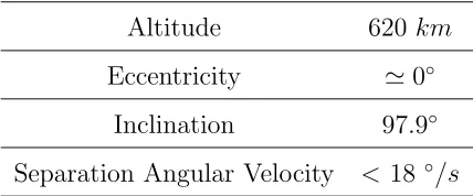
Table 1: UniSat-6 orbital parameters at the injection

Altitude 620 km

Eccentricity _≃0◦

Inclination 97.9◦

Separation Angular Velocity <18 ◦_/s

UniSat-6 main task was the in orbit release of the boarded CubeSats. The released spacecrafts were Tigrisat (3U), Lemur-1 (3U), AntelSat (2U) and Aerocube 6 (1U) for a total deployment volume capability of 9U. The deploy-ment of the satellites took place 25 hours and 38 minutes after the launch and it was initiated by an autonomous system with a dedicated battery. Confirmation of the deployment was given 15 minutes after release when the spacecraft passed the over ground station in Italy. All the deployed CubeSats communicated with ground, confirming the good health of all the satellites and the full accomplishment of the deployment operations [18].

The ground station in Roma managed to establish a two ways effective com-munication with it few minutes after launch. [19].

2.3. ADCS hardware

UniSat-6 is equipped with various devices for attitude determination and control. Attitude related measurements are given by two sensors, a rate gyro (L3GD20) and a magnetometer (HMC5883L). The L3GD20 is a low-power MEMS three-axis angular rate sensor, used in terrestrial applications such as video-games, GPS navigation and robotics. The HMC5883L is a three-axis compass that enables 1◦ _{to 2}◦ _{compass heading accuracy.}

UniSat-6 does not have an active attitude control, but relies on a passive magnetic control to stabilize the spacecraft. Since UniSat-6 does not have strict requirements on pointing, the choice of passive magnetic control is a good compromise between simplicity, cost and performances. The magnetic torque is generated by 4 permanent magnets and 17 hysteresis rods. The magnets are made of Alnico-5 and give a total magnetic dipole of 5 Am2_.

They are placed along the ˆyb axis of the satellite. The 17 hysteresis rods are

spread on the 3 axes: 8 along the ˆxb axis, 1 along the ˆyb axis and other 8

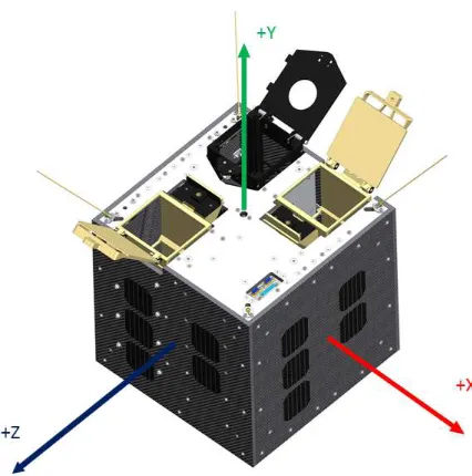
along the ˆzb axis. Fig. 1 shows the position of these devices on board of

Figure 1: Position of magnets and hysteresis rods (magnetometers defined axes)

3. Attitude determination

3.1. Reference frames

In order to represent the orientation of the spacecraft, three reference frames are introduced. The first reference frame _Cˆ_{1 C}ˆ_{2 C}ˆ₃ is an Earth Centred Earth Fixed (ECEF) frame. The first two axes are contained in the equatorial plane of the Earth, with the first directed from the centre of the Earth to the Greenwich meridian. The third axis is directed from the centre of the Earth to the North Pole. The second axis completes the orthogonal reference frame.

The second reference frame rˆ θˆ ˆh

velocity of the orbit. The third axis is directed along the perpendicular to the orbital plane.

The third reference frame xˆb yˆb zˆb

is the body-axes reference frame, represented in Fig. 3. The reference frame has its origin in the centre of mass of the spacecraft. The ˆxb and ˆzb axes exit from the side panels of the

space-craft. The ˆyb is pointing towards the direction of the release of the CubeSats

(i.e. parallel to the deployers). This reference frame is different from the one shown in Fig. 1, which is related to the inner axes of the magnetometer. The aim of this paper is to analyze the orientation of the body frame with respect to the orbital frame because the latter constitutes the main refer-ence frame for the analysis of spacecraft attitude control algorithms. This orientation is easily expressed by means of the Euler angles φ, θ, ψ in the sequence 3-2-1, defined as in Fig. 2. In order to obtain the Euler angles, the orientation of the ECEF frame with respect to the orbital frame and the orientation of the body frame with respect to the ECEF frame need to be calculated. The orientation of the ECEF frame with respect to the orbital frame is given by three successive rotations as follows:

1. a rotation about the ˆC3axis of the ECEF frame by the Right Ascension

of the Ascending Node (RAAN) Ω

2. a rotation about the new ˆC1’ axis by the argument of latitude u

Figure 2: Euler angles and orbital frame

The rotation matrix that represents the orientation is given by the multipli-cation of the three rotation matrices T1, T2, T3.

     ˆ C1 ˆ C2 ˆ C3      =T      ˆ r ˆ θ ˆ h     

=T1T2T3

     ˆ r ˆ θ ˆ h      (1)

T1 =

    

cos Ω ₋sin Ω 0 sin Ω cos Ω 0

0 0 1

     (2)

T2 =

    

1 0 0

0 cosi ₋sini

0 sini cosi

     (3)

T3 =

    

cosu ₋sinu 0 sinu cosu 0

0 0 1

     (4)

The argument of latitude u is calculated as the sum of the true anomaly ν

and the argument of perigee ̟:

u=ν+̟ (5)

The orientation of the body frame with respect to the inertial frame is given by a quaternion, which is calculated by the filter that will be presented in Section 3.4.

3.2. Attitude representation and kinematics

will be introduced.

The attitude representation employed by the filter to represent the orienta-tion from the ECEF frame to the body frame is dual. A quaternion repre-sentation is used to express the input, the output and the kinematic model inside the filter. A vector of generalized Rodrigues parameters is used in some numerical operations of the filter that might violate the unity norm property of the quaternion, otherwise.

The quaternion q is defined as

q= q1 q2 q3 q4

′

= q q¯ 4

′

(6)

The kinematic equation associated to the quaternion is given by

˙

q= 1

2Ξ(q(t))ω(t) (7) where ω is the angular velocity vector of the satellite and Ξ is a matrix defined as

Ξ(q) =  

q4I3×3+ ¯q× −q¯T



 (8)

where ¯q_× is the cross-product matrix associated to the vector ¯q. Given the discrete-time nature of the application studied in this paper, a discrete-time version of Eq. 7 has to be introduced. The quaternion at the k+ 1th _{step of}

the algorithm is

qk+1 = Ω(ωk)qk (9)

with

Ω(ωk) =

 

Zk ψk

−ψk cos (0.5kωkk∆t)

 

Zk = cos (0.5kωkk∆t)I3×3−ψk×

ψk = sin (0.5kω

kk∆t)ωk

kωkk

where ωk is the angular velocity vector, measured from the rate-gyros, and

∆t the measurements sampling interval.

The quaternion is used to express the orientation of the body frame with respect to the orbital frame. This is done by defining a direction cosine matrix DCM equivalent to the quaternion and multiplying it by the T ma-trix defined in Eq. 1. The direction cosine mama-trix DCM obtained from a quaternion q is calculated as

DCM =     

1₋2(q2

2 +q32) 2(q1q2+q3q4) 2(q1q3−q2q4)

2(q1q2−q3q4) 1−2(q12+q32) 2(q2q3+q1q4)

2(q1q3 +q2q4) 2(q2q3−q1q4) 1−2(q22+q22)

    

(11)

A four-components quaternions is a non-singular representation of the special orthogonal group SO(3) of three-dimensional rotation matrices which repre-sents 3D attitude and it is therefore a redundant representation [20]. The multiplicative quaternion approach, commonly used in spacecraft attitude estimation problems, adopts this redundancy to represent the reference atti-tude free of singularity while the three components representation describes the deviation from this reference [21]. Therefore, the algorithm represents the attitude as the quaternion product

¯

q=δq(~v)_×q¯ref

δq= δq δq¯ 4

(12)

where ¯qref is the reference quaternion and the small deviationδq(a) from ¯qref

to the actual attitude q is parameterized by a three-component vector ~v. The error quaternion components are used to define the vector of generalized Rodrigues parameters δp

δp=f δq¯ a+δq4

where the parameter a _∈ h 0 1 i

and f is a scale factor. For a = 0 and

f = 1, Eq. 13 returns the Gibbs vector, while for a = 1 and f = 1 it gives the standard modified Rodrigues parameters. According to [11], the choice of f = 2(a+ 1) is a suitable pick and it will be adopted throughout this paper.

The inverse transformation from δp toδq is

δq4 =

−akδpk2

+f√f2_+(1−a2_)kδpk2 f2_+kδpk2

δq¯=f−1_(a+δq 4)δp

(14)

3.3. Measurements model

The available measurements on board Unisat-6 are the Earth magnetic field vector from the magnetometer and the spacecraft angular velocity vector from the rate-gyros.

The magnetometer measures the intensity of the Earth magnetic field along its three axes (see Fig. 1), that can be easily translated into the body axes (see Fig. 3). This vector can be compared with the information of the World Magnetic Model (WMM), which returns the intensity of the Earth magnetic field in the ECEF frame, thus giving information on the orientation of the body axes frame with respect to the ECEF frame. The noise on the measurement vector ~b of the magnetometer is modeled as an additive Gaussian zero-mean white process with variance σm.

The rate-gyro measures the angular velocity ω of the satellite in the body frames. This measurement is usually modeled as [22]

˜

ω(t) =ωtrue(t) +β(t) +ηv(t)

˙

β(t) =ηu(t)

where the true angular velocity ωtrue is corrupted by a bias β, and ηv and

ηu are two Gaussian zero-mean white processes with variances σv and σu,

respectively.

3.4. Unscented attitude filter

The filter employed for UniSat-6 attitude reconstruction was first pro-posed in [11] and it was given the name of USQUE (UnScented QUaternion Estimator, which is also a Latin expression meaning ‘all the way’). The USQUE is an attitude-dedicated formulation of the Unscented filter. This section will present the algorithm of the filter employed in this work.

The USQUE, as well as the original formulation of the Unscented filter, is constituted by a prediction phase, in which the a priori estimate is con-structed by averaging the values of a finite number of points from the state space (the σ-points), and by a correction phase, in which the a priori esti-mate is corrected with the information from the measurements. The USQUE algorithm employs the data from the rate-gyro in the prediction phase so as to calculate the kinematics of the satellite, while the magnetometer output is the only measurement employed in the correction phase.

The algorithm described in the following assumes a discrete-time nonlinear system, modeled as

xk+1 =f(xk, k) +Gkwk

˜

yk=h(xk,k) +vk

(16)

where xk is the state vector, ˜yk is the measurement vector, and wk and vk

are zero-mean Gaussian noise vectors representing the process noise and the measurements noise with covariance matrices Qk and Rk, respectively.

parameters and the biases of the rate-gyros.

ˆ

x=  

δp β



 (17)

A quaternion can serve as an initial guess for the attitude, since it can be transformed into the vector of generalized Rodrigues parameters with Eq. 13. The filter is initialized with an initial guess for the state estimate ˆx and an initial value for the error covariance matrix P.

The algorithm starts with a step of the prediction phase. The σ-points at the kth _{step are defined as:}

χk =

 

χδp_k (i)

χβ_k(i) 

, i= 0,1, . . . ,2n (18)

with n being the size of the state vector. In the σ-points partitioning, χδp_k

represents the attitude-error part and χβ_k the gyro bias part. The 2n + 1

σ-points depend on the actual value of the estimated state ˆx+_k and of the error covariance matrix P_k+ and are chosen from the columns of the matrix

M:

M = ˆx+k +

h

0n S −S

i

S =p(n+λ)(P_k++Qk)

(19)

in which λ is a tuning parameter of the filter which tells how much the σ -points are spread around the mean. In order to propagate the attitude, the

χδp_k are transformed into correspondent quaternion deviationsδq+

k, by means

of Eq. 14. These deviations are used as in Eq. 12 to form a set of attitude quaternions spread around the mean ˆq+

k. The resulting set is

ˆ

q_k+(0) = ˆq+_k

ˆ

The first of these equations implies thatχδp_k (0) be zero. Therefore, this reset is to be performed at each step of the algorithm.

Once that the quaternion representation of theσ-points has been calculated, the attitude can be propagated using the discrete kinematics of Eq. 9, where the angular velocity to be used is the estimated quantity ˆω_k+:

ˆ

ω+_k(i) = ˜ωk−χ β

k(i), i= 0,1, . . . ,2n (21)

After the propagation of the quaternions, the propagated Rodrigues param-eters can be obtained back by using Eq. 13, where the error quaternions are obtained once again by applying Eq. 12. At the end of the prediction phase, the propagated σ-points are

χδp_k+1(0) = 0

χδp_k+1(i) =f δ¯q−k+1(i) a+δq−

4k+1(i)

, i= 1,2, . . . ,2n χβ_k+1(i) = χβk(i), i= 0,1, . . . ,2n

(22)

The predicted state vector ˆx−_k+1 is computed as

ˆ

x−_k+1 = 1

n+λ

(

λχk+1(0) +

1 2

2n

X

i=1

χk+1(i)

)

(23)

The predicted error covariance matrix is calculated as

P_k+1− = 1

n+λ

n

λ

χk+1(0)−xˆ−_k+1 χk+1(0)−xˆ−_k+1

T (24) +1 2 2n X i=1

χk+1(i)−xˆ−k+1 χk+1(i)−xˆ−k+1

T )

+Qk

The mean observation is given by

ˆ

y_k+1− = 1

n+λ

(

λγk+1(0) + +

1 2

2n

X

i=1

γk+1(i)

)

where γk+1(i) are the measurements obtained by applying the h function

from Eq. 16 to the set χk+1(i).

The innovation covariance matrix is given by

Pνν k+1 =

1

n+λ

n

λ

γk+1(0)−yˆ_k+1− γk+1(0)−yˆ−_k+1

T (26) +1 2 2n X i=1

γk+1(i)−yˆk+1− γk+1(i)−yˆk+1−

T )

+Rk+1

The cross-correlation matrix is given by

P_k+1xy = 1

n+λ

n

λ

χk+1(0)−xˆ−k+1 γk+1(0)−yˆk+1−

T (27) +1 2 2n X i=1

χk+1(i)−xˆ−k+1 γk+1(i)−yˆk+1−

T )

The correction phase consists in the update of the predicted state vectorx−_k+1

and of the error covariance matrix P_k+1−

ˆ

x+_k+1 = ˆx−_k+1+Kkvk (28)

P_k+1+ =P_k+1− ₋KkPkvvK T

k (29)

where vk is the innovation and Kk the Kalman gain, given by, respectively

vk = ˜yk−h(ˆx−k, k) (30)

Kk =P xy k (P

νν k )

−1

(31) The process noise covariance matrix Qkis actualized at each time step, since

the measurements sampling time is not constant. According to [11], the matrix is defined as

Qk=

∆t

2  

(σ2 v− 16σ

2

u∆t2)I3×3 03×3

03×3 σu2I3×3



 (32)

At the kth _{step the filter provides the estimation vector ˆx}

k and the matrix

4. Results

This section describes the results of attitude reconstruction performed starting from the UniSat-6 flight data as received by the GAUSS ground sta-tion in Roma. These data include telemetry of the satellite and data from the sensors that were stored along a time interval of more than 26 hours, which corresponds to approximately 18 orbits of UniSat-6 around the Earth. These operations were performed on April 24th-25th, 2015 with the initial time instant t0 at 20:51 UTC of April 24th. Data sampling rate is variable, since the on-board computer does not give a clock for the measurements. Most of the measurements occur with a time interval of 4-6 seconds.

The initial guess for the attitude corresponds to the first measurement from the magnetometers, while a value of 0.1_·π/180 is assumed for the three gyro biases. The error covariance matrixP is initialized with the variances of the magnetometers and of the gyro biases. The value ofλ was chosen to be equal to 0.05.

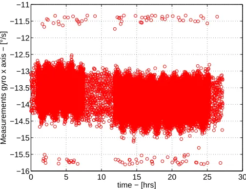
Fig. 4 shows the measurements history from the ˆxb axis rate-gyro. It can be

seen that, during the considered time interval, there are two periods in which measurements are much more frequent (areas in which circles are denser). At

t0, UniSat-6 was in a normal operation mode with data sampling every 30

sec-onds. A high-frequency measurements mode was set up for UniSat-6 almost an hour after t0, at 21:44 UTC. Six hours later, at 4:18 UTC, the satellite

0 5 10 15 20 25 30 −16

−15.5 −15 −14.5 −14 −13.5 −13 −12.5 −12 −11.5 −11

Measurements gyro x axis − [°/s]

time − [hrs]

Figure 4: ˆxb axis gyro measurements

22:10 UTC. A normal operation mode interval closes the sequence of data until 0:00 UTC.

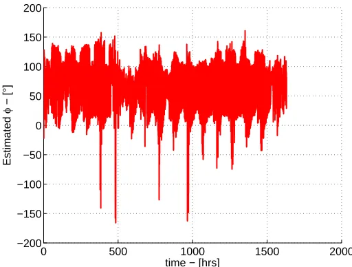
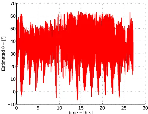
Figs. 5 and 6 show the results of the estimated Euler angles of roll ( ˆφ) and pitch (ˆθ). These angles, as well as the yaw angle ( ˆψ) that will be analyzed later, are obtained by transforming the quaternion calculated as output of the filter with the procedure described in Section 3.2. The superimposed ˆ symbol indicates that these variables are estimated.

It can be seen that ˆφ and ˆψ angles oscillate within a certain range of values. The roll angle varies mainly between 0◦ _{and 100}◦_{. The pitch angle varies}

mainly between 0◦ _{and 60}◦_{. These rotations are very fast, in the order of 4-5}

0 500 1000 1500 2000 −200

−150 −100 −50 0 50 100 150 200

Estimated

φ

− [°]

time − [hrs]

Figure 5: Estimated φangle

aperture of the cone is variable.

Comparing the results of Fig. 6 with those of Fig. 4, it can be seen that the amplitude of the periodical variations is diminished when the satellite goes in the normal operation mode. The results of attitude reconstruction are degraded with this mode. This is reasonable, since these measurements have a higher sampling time although the satellite is still rotating fast. Neverthe-less, the algorithm is still able to satisfactorily estimate the attitude of the satellite. Furthermore, the degradation of the results is visible only in the reconstruction of the pitch angle. This is a first indication of the robustness of the filter.

0 5 10 15 20 25 30 −10

0 10 20 30 40 50 60 70

Estimated

θ

− [°]

time − [hrs]

Figure 6: Estimated θ angle

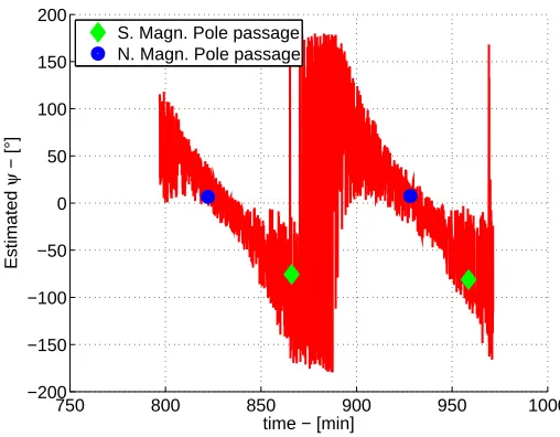
between -180◦ _{and 180}◦_{. Fig. 8 shows a sample of the ˆψ history}

concern-ing two consecutive orbits. In particular, the selected orbits pass over the North and South magnetic poles with the closest approximation among all the considered orbits. The circles and the diamonds approximately indicate the passages over the North and the South Magnetic Pole, respectively. Re-membering that, by definition, the yaw angle defined in Fig. 2 is the angle between ˆrand the projection of ˆxb on the orbital plane, an interesting result

about the attitude motion can be derived.

At the passage over the North magnetic pole (located at approximately 80◦

of latitude North), it can be seen that the value of ˆψ is close to zero. This means that the projection of the ˆxb axis is almost aligned to the orbit radius.

0 5 10 15 20 25 30 −200

−150 −100 −50 0 50 100 150 200

Estimated

ψ

− [°]

time − [hrs]

Figure 7: Estimated ψ angle

750 800 850 900 950 1000

−200 −150 −100 −50 0 50 100 150 200

Estimated

ψ

− [°]

time − [min] S. Magn. Pole passage N. Magn. Pole passage

orbital plane, is aligned with the lines of the Earth magnetic field.

Continuing towards the South magnetic pole, the value of ˆψ decreases slowly, until it reaches almost -90◦_{right before reaching the South magnetic pole}

(lo-cated at approximately -60◦ _{of latitude South). Right after the passage over}

the South magnetic pole, the value of ˆψ passes abruptly from -90◦ _{to -180}◦

and rises eventually to 180◦_{. After reaching the 180}◦ _{halfway the path from}

the South to the North magnetic pole, ˆψ starts decreasing again, until it reaches a value of almost 0◦ _{over the North magnetic pole.}

This behavior suggests that the ˆxb axis has been aligned to the lines of the

Earth magnetic field due to the magnetization of the hysteresis rod along ˆxb.

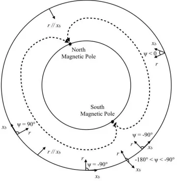
A perfect alignment with the lines of the Earth magnetic field would have implied ψ = ₋180◦ _{above the South magnetic pole (lines of the magnetic}

field going out from the Earth – see also Fig. 9). Nevertheless, the use of a passive magnetic attitude control system does not guarantee this perfect alignment, but only a coarse one. Furthermore, because of the not symmetric distribution of the magnetic poles on the surface of the Earth, the path from the North to the South magnetic pole is shorter than the one from South to North for the considered orbits. Therefore, when traveling from North to South, the ˆxb axis has less time to complete the -180◦ rotation of the lines of

the Earth magnetic field. This is why the spacecraft experiences a big yaw rotation right after the passage above the South magnetic pole.

The contribution of the other magnetic devices (permanent magnets along ˆ

yb, hysteresis rods along ˆyb and ˆzb) can be neglected. The contribution of

the hysteresis rod along the ˆyb axis is equivalent only to 1/8 of the effect of

Figure 9: Yaw orientation along the orbit

hysteresis rods along the ˆzb axis are not effective. The average effect of the

magnetic torque produced by them, calculated on a full rotation, is, in fact, zero. Since the rotations of roll and pitch are much faster than those of yaw (3-5 rpm against 0.01 rpm), the average torque of the formers goes rapidly to zero. In order for the devices along ˆyb and ˆzb to work, UniSat-6 should

have been equipped with a detumbling control to stop the initial rotations. A small variation in the amplitude of the yaw variation can be seen in the fifth orbit of Fig. 7, when the yaw arrives only at 160◦ _{and not at 180}◦_{. This}

is in correspondence with the normal operation mode when there available measurements have a higher sampling time.

In conclusion, the attitude motion of UniSat-6 is composed of two dynamics, a long period one and a short period one. The long period motion consists of two 360◦ _{yaw rotations completed in one orbit, which makes the ˆx}

b axis

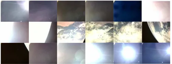
Figure 10: 25 s sequence of pictures from the on-board camera

the fast oscillations (up to 5rpm) of roll and pitch, which describe a variable aperture elliptical cone in space.

These data are consistent with the images taken from the camera of UniSat-6, placed on top the ˆyb panel. Several images were taken both in the direction

of the Earth and in the direction of the outer space, as it is shown in Fig. 10. This figure is composed of 18 pictures taken from the camera between April 25, 2015 10:17:29 UTC and April 25, 2015 10:17:54 UTC. In the first picture, the camera is pointing towards the Sun; then, it is pointing towards the Earth (pictures 7 to 13); eventually, it points towards the Sun again. The panel with the camera (ˆyb axis), therefore, describes a cone in space.

5. Conclusions

This paper has presented the results of the attitude determination of the UniSat-6 satellite. The estimation was realized analyzing real data collected on-board the spacecraft and processed at ground.

its ˆxb axis to the lines of the Earth magnetic field, while the two other axes

rotate in space with a period of 5 rpm.

Due to a problem on the on-board electronics caused by a radiation event, the spacecraft was not able to collect data with the expected sampling rate (30 s instead of 4 s) for six hours. Nevertheless, in this interval the filter was able to reconstruct the attitude of the spacecraft with almost the same accuracy as before. The reconstructed attitude of the spacecraft is consistent with the images taken from the on-board camera.

References

[1] J. A. Vil´an, F. Aguado Agelet, M. L´opez Est´evez, A. Gonz´alez Mui˜no, Flight results: Reliability and lifetime of the polymeric 3d-printed an-tenna deployment mechanism installed on xatcobeo & humsat-d, Acta Astronautica 107 (2015) 290–300.

[2] B. Malphrus, M. Combs, J. Kruth, K. Brown, B. Twiggs, E. Thomas, T. Rose, University-based nanosatellite missions and ground operations at morehead state.

[3] A. Nascetti, E. Pittella, P. Teofilatto, S. Pisa, High-gain s-band patch antenna system for earth-observation cubesat satellites, Antennas and Wireless Propagation Letters, IEEE 14 (2015) 434–437.

[5] B. Klofas, Upcoming amateur radio cubesats: The flood has arrived, Paper presented at the 2013 AMSAT Annual Meeting and Space Sym-posium, Houston, Texas, USA (2013).

[6] B. Klofas, Cubesat communications update, Paper presented at the CubeSat 2014 Summer Workshop, Logan, Utah, USA (2014).

[7] C. Paris, M. Parisse, A. Nascetti, R. Cica, N. A. Salman, The tigrisat camera a nanosatellite optical payload for detecting dust and sand storms, in: Environment and Electrical Engineering (EEEIC), 2015 IEEE 15th International Conference on, IEEE, 2015, pp. 1605–1610.

[8] J. L. Crassidis, F. L. Markley, Y. Cheng, Survey of nonlinear attitude estimation methods, Journal of Guidance, Control, and Dynamics 30 (1) (2007) 12–28.

[9] J. L. Farrell, Attitude determination by kalman filtering, Automatica 6 (3) (1970) 419–430.

[10] E. J. Lefferts, F. L. Markley, M. D. Shuster, Kalman filtering for space-craft attitude estimation, Journal of Guidance, Control, and Dynamics 5 (5) (1982) 417–429.

[11] J. L. Crassidis, F. L. Markley, Unscented filtering for spacecraft attitude estimation, Journal of guidance, control, and dynamics 26 (4) (2003) 536–542.

[13] P. Sekhavat, Q. Gong, I. Ross, Unscented kalman filtering: Npsat1 ground test results, in: AIAA Guidance, Navigation, and Control Con-ference, Keystone, Colorado, 2006.

[14] J.-W. Kim, J. L. Crassidis, S. R. Vadali, A. Dershowitz, International space station leak localization using attitude response data, Journal of guidance, control, and dynamics 29 (5) (2006) 1041–1050.

[15] G. Figueir´o de Oliveira, P. H. D´oria Nehme, C. Cappelletti, Analysis and simulation of attitude determination and control for the serpens nanosatellite, in: Proceedings of the 2nd IAA Conference on Dynamics and Control of Space Systems, International Academy of Astronautics, 2014.

[16] A. Nascetti, D. Pancorbo-D’Ammando, M. Truglio, Abacus advanced board for active control of university satellites, in: Proceedings of the 2nd IAA Conference on University Satellite Missions and Cubesat Work-shop, International Academy of Astronautics, 2013.

[17] S. Paiano, M. Truglio, A. Conde Rodriguez, C. Cappelletti, F. Graziani, Unisat-6 mission, in: Proceedings of the 1st Latin American IAA Cube-sat Workshop, International Academy of Astronautics, 2014.

[19] A. Conde Rodriguez, M. Truglio, F. Graziani, C. Cappelletti, Mi-crosatellites ground operations and best practices from the experience of unisat-6, in: Proceedings of the 66th International Astronautical Congress, International Astronautical Federation, 2015.

[20] F. L. Markley, Multiplicative vs. additive filtering for spacecraft attitude determination, in: Proceedings of the 6th Conference on Dynamics and Control of Systems and Structures in Space (DCSSS), Vol. 22, 2004.

[21] F. L. Markley, Attitude error representations for kalman filtering, Jour-nal of guidance, control, and dynamics 26 (2) (2003) 311–317.