Commonsense Knowledge Base Completion
Xiang Li∗‡ Aynaz Taheri† Lifu Tu‡ Kevin Gimpel‡ ∗University of Chicago, Chicago, IL, 60637, USA †University of Illinois at Chicago, Chicago, IL, 60607, USA ‡Toyota Technological Institute at Chicago, Chicago, IL, 60637, USA
[email protected],[email protected],{lifu,kgimpel}@ttic.edu
Abstract
We enrich a curated resource of common-sense knowledge by formulating the prob-lem as one of knowledge base comple-tion (KBC). Most work in KBC focuses on knowledge bases like Freebase that re-late entities drawn from a fixed set. How-ever, the tuples in ConceptNet (Speer and Havasi, 2012) define relations between an unbounded set of phrases. We develop neural network models for scoring tuples on arbitrary phrases and evaluate them by their ability to distinguish true held-out tuples from false ones. We find strong performance from a bilinear model using a simple additive architecture to model phrases. We manually evaluate our trained model’s ability to assign quality scores to novel tuples, finding that it can propose tu-ples at the same quality level as medium-confidence tuples from ConceptNet.
1 Introduction
Many ambiguities in natural language process-ing (NLP) can be resolved by usprocess-ing knowledge of various forms. Our focus is on the type of knowledge that is often referred to as “common-sense” or “background” knowledge. This knowl-edge is rarely expressed explicitly in textual cor-pora (Gordon and Van Durme, 2013). Some re-searchers have developed techniques for inferring this knowledge from patterns in raw text (Gor-don, 2014; Angeli and Manning, 2014), while oth-ers have developed curated resources of common-sense knowledge via manual annotation (Lenat and Guha, 1989; Speer and Havasi, 2012) or games with a purpose (von Ahn et al., 2006).
Curated resources typically have high preci-sion but suffer from a lack of coverage. For
cer-relation right term conf.
MOTIVATEDBYGOAL relax 3.3
USEDFOR relaxation 2.6
MOTIVATEDBYGOAL your muscle be sore 2.3 HASPREREQUISITE go to spa 2.0
CAUSES get pruny skin 1.6
[image:1.595.309.526.220.294.2]HASPREREQUISITE change into swim suit 1.6 Table 1: ConceptNet tuples with left term “soak in hotspring”; final column is confidence score.
tain resources, researchers have developed meth-ods to automatically increase coverage by infer-ring missing entries. These methods are com-monly categorized under the heading of knowl-edge base completion (KBC). KBC is widely-studied for knowledge bases like Freebase (Bol-lacker et al., 2008) which contain large sets of enti-ties and relations among them (Mintz et al., 2009; Nickel et al., 2011; Riedel et al., 2013; West et al., 2014), including recent work using neural net-works (Socher et al., 2013; Yang et al., 2014).
We improve the coverage of commonsense re-sources by formulating the problem as one of knowledge base completion. We focus on a par-ticular curated commonsense resource called Con-ceptNet (Speer and Havasi, 2012). ConCon-ceptNet contains tuples consisting of a left term, a rela-tion, and a right term. The relations come from a fixed set. While terms in Freebase tuples are en-tities, ConceptNet terms can be arbitraryphrases. Some examples are shown in Table 1. An NLP ap-plication may wish to query ConceptNet for infor-mation about soaking in a hotspring, but may use different words from those contained in the Con-ceptNet tuples. Our goal is to do on-the-fly knowl-edge base completion so that queries can be an-swered robustly without requiring the precise lin-guistic forms contained in ConceptNet.
To do this, we develop neural network mod-els to embed terms and provide scores to
trary tuples. We train them on ConceptNet tuples and evaluate them by their ability to distinguish true and false held-out tuples. We consider sev-eral functional architectures, comparing two com-position functions for embedding terms and two functions for converting term embeddings into tu-ple scores. We find that all architectures are able to outperform several baselines and reach similar performance on classifying held-out tuples.
We also experiment with several training ob-jectives for KBC, finding that a simple cross en-tropy objective with randomly-generated negative examples performs best while also being fastest. We manually evaluate our trained model’s abil-ity to assign qualabil-ity scores to novel tuples, find-ing that it can propose tuples at the same qual-ity level as medium-confidence tuples from Con-ceptNet. We release all of our resources, includ-ing our ConceptNet KBC task data, large sets of randomly-generated tuples scored with our model, training code, and pretrained models with code for calculating the confidence of novel tuples.1
2 Related Work
Our methods are similar to past work on KBC (Mintz et al., 2009; Nickel et al., 2011; Lao et al., 2011; Nickel et al., 2012; Riedel et al., 2013; Gardner et al., 2014; West et al., 2014), particu-larly methods based on distributed representations and neural networks (Socher et al., 2013; Bordes et al., 2013; Bordes et al., 2014a; Bordes et al., 2014b; Yang et al., 2014; Neelakantan et al., 2015; Gu et al., 2015; Toutanova et al., 2015). Most prior work predicts new relational links between terms drawn from a fixed set. In a notable exception, Neelakantan and Chang (2015) add new entities to KBs using external resources along with prop-erties of the KB itself. Relatedly, Yao et al. (2013) induce an unbounded set of entity categories and associate them with entities in KBs.
Several researchers have developed techniques for discovering commonsense knowledge from text (Gordon et al., 2010; Gordon and Schu-bert, 2012; Gordon, 2014; Angeli and Manning, 2014). Open information extraction systems like REVERB (Fader et al., 2011) and NELL
(Carl-son et al., 2010) find tuples with arbitrary terms and relations from raw text. In contrast, we start with a set of commonsense facts to use for
train-1Available at http://ttic.uchicago.edu/
˜kgimpel/commonsense.html.
ing, though our methods could be applied to the output of these or other extraction systems.
Our goals are similar to those of the Analogy-Space method (Speer et al., 2008), which uses ma-trix factorization to improve coverage of Concept-Net. However, AnalogySpace can only return a confidence score for a pair of terms drawn from the training set. Our models can assign scores to tuples that contain novel terms (as long as they consist of words in our vocabulary).
Though we use ConceptNet, similar techniques can be applied to other curated resources like WordNet (Miller, 1995) and FrameNet (Baker et al., 1998). For WordNet, tuples can contain lexi-cal entries that are linked via synset relations (e.g., “hypernym”). WordNet contains many multi-word entries (e.g., “cold sweat”), which can be modeled compositionally by our term models; al-ternatively, entire glosses could be used as terms. To expand frame relationships in FrameNet, tuples can draw relations from the frame relation types (e.g., “is causative of”) and terms can be frame lexical units or their definitions.
Several researchers have used commonsense knowledge to improve language technologies, in-cluding sentiment analysis (Cambria et al., 2012; Agarwal et al., 2015), semantic similarity (Caro et al., 2015), and speech recognition (Lieberman et al., 2005). Our hope is that our models can en-able many other NLP applications to benefit from commonsense knowledge.
Our work is most similar to that of Angeli and Manning (2013). They also developed methods to assess the plausibility of new facts based on a training set of facts, considering commonsense data from ConceptNet in one of their settings. Like us, they can handle an unbounded set of terms by using (simple) composition functions for novel terms, which is rare among work in KBC. One key difference is that their best method requires iterat-ing over the KB at test time, which can be com-putationally expensive with large KBs. Our mod-els do not require iterating over the training set. We compare to several baselines inspired by their work, and we additionally evaluate our model’s ability to score novel tuples derived from both ConceptNet and Wikipedia.
3 Models
as-sume this knowledge is given in the form of tuples ht1, R, t2i, wheret1is theleft term,t2is theright
term, andRis a (directed)relationthat exists be-tween the terms. Examples are shown in Table 1.2
Given a set of tuples, our goal is to develop a parametric model that can provide a confidence score for new, unseen tuples. That is, we want to design and train models that define a function score(t1, R, t2) that provides a quality score for
an arbitrary tupleht1, R, t2i. These models will be
evaluated by their ability to distinguish true held-out tuples from false ones.
We describe two model families for scoring tu-ples. We assume that we have embeddings for words and define models that use these word em-beddings to score tuples. So our models are lim-ited to tuples in which terms consist of words in the word embedding vocabulary, though future work could consider character-based architectures for open-vocabulary modeling (Huang et al., 2013; Ling et al., 2015).
3.1 Bilinear Models
We first consider bilinear models, since they have been found useful for KBC in past work (Nickel et al., 2011; Jenatton et al., 2012; Garc´ıa-Dur´an et al., 2014; Yang et al., 2014). A bilinear model has the following form for a tupleht1, R, t2i:
v>1MRv2
wherev1 ∈Rris the (column) vector representing
t1,v2 ∈ Rris the vector fort2, andMR ∈ Rr×r
is the parameter matrix for relationR.
To convert termst1 andt2 into term vectorsv1
andv2, we consider two possibilities: word
aver-aging and a bidirectional long short-term memory (LSTM) recurrent neural network (Hochreiter and Schmidhuber, 1997). This provides us with two models:Bilinear AVGandBilinear LSTM.
One downside of this architecture is that as the length of the term vectors grows, the size of the re-lation matrices grows quadratically. This can slow down training while requiring more data to learn the large numbers of parameters in the matrices. To address this, we include an additional nonlin-ear transformation of each term:
ui=a(W(B)vi+b(B))
2These examples are from the Open Mind Common Sense (OMCS) part of ConceptNet version 5 (Speer and Havasi, 2012). In our experiments below, we only use OMCS tuples.
wherea is a nonlinear activation function (tuned among ReLU, tanh, and logistic sigmoid) and where we have introduced additional parameters
W(B)andb(B). This gives us the following model:
scorebilinear(t1, R, t2) =u>1MRu2
When using the LSTM, we tune the decision about how to produce the final term vectors to pass to the bilinear model, including possibly using the final vectors from each direction and the output of max or average pooling. We use the same LSTM pa-rameters for each term.
3.2 Deep Neural Network Models
Our second family of models is based on deep neu-ral networks (DNNs). While bilinear models have been shown to work well for KBC, their functional form makes restrictions about how terms can inter-act. DNNs make no such restrictions.
As above, we define two models, one based on using word averaging for the term model (DNN AVG) and one based on LSTMs (DNN LSTM). For the DNN AVG model, we obtain the term vec-torsv1andv2by averaging word vectors in the
re-spective terms. We then concatenatev1,v2, and a
relation vectorvR to form the input of the DNN, denotedvin. The DNN uses a single hidden layer:
u=a(W(D1)vin +b(D1))
scoreDNN(t1, R, t2) =W(D2)u+b(D2) (1)
where a is again a (tuned) nonlinear activation function. The size of the hidden vector u is tuned, but the output dimensionality (the numbers of rows inW(D2) andb(D2)) is fixed to 1. We do
not use a nonlinear activation for the final layer since our goal is to output a scalar score.
For the DNN LSTM model, we first create a single vector for the two terms using an LSTM. That is, we concatenatet1, a delimiter token, and
t2to create a single word sequence. We use a
bidi-rectional LSTM to convert this word sequence to a vector, again possibly using pooling (the deci-sion is tuned; details below). We concatenate the output of this bidirectional LSTM with the rela-tion vectorvrto create the DNN input vectorvin,
The relation vectorsvR are learned in addition
to the DNN parameters W(D1), W(D2), b(D1),
b(D2), and the LSTM parameters (in the case of
the DNN LSTM model). Also, word embedding parameters are updated in all settings.
4 Training
Given a tuple training setT, we train our models using two different loss functions: hinge loss and a binary cross entropy function. Both rely on ways of generating negative examples (Section 4.3). Both also use regularization (Section 4.4).
4.1 Hinge Loss
Given a training tuple τ = ht1, R, t2i, the hinge
loss seeks to make the score of τ larger than the score of negative examples by a margin of at least
γ. This corresponds to minimizing the following loss, summed over all examplesτ ∈T:
losshinge(τ) =
max{0, γ−score(τ) + score(τneg(t1))} + max{0, γ−score(τ) + score(τneg(R))}
+ max{0, γ−score(τ) + score(τneg(t2))}
whereτneg(t1)is the negative example obtained by
replacingt1 inτ with some othert1, and τneg(R)
andτneg(t2) are defined analogously for the rela-tion and right term. We describe how we generate these negative examples in Section 4.3 below.
4.2 Binary Cross Entropy
Though we only have true tuples in our training set, we can create a binary classification problem by assigning a label of 1 to training tuples and a label of 0 to negative examples. Then we can min-imize cross entropy (CE) as is common when us-ing neural networks for classification. To generate negative examples, we consider the methods de-scribed in Section 4.3 below. We also need to con-vert our models’ scores into probabilities, which we do by using a logistic sigmoidσonscore. We denote the label as`, where the label is 1 if the tu-ple is from the training set and 0 if it is a negative example. Then the loss is defined:
lossCE(τ, `) =
−`logσ(score(τ))−(1−`) log(1−σ(score(τ))) When using this loss, we generate three negative examples for each positive example (one for swap-ping each component of the tuple, as in the hinge
loss). For a mini-batch of sizeβ, there areβ pos-itive examples and3βnegative examples used for training. The loss is summed over these4β exam-ples yielded by each mini-batch.
4.3 Negative Examples
For the loss functions above, we need ways of au-tomatically generating negative examples. For ef-ficiency, we consider using the current mini-batch only, as our models are trained using optimiza-tion on mini-batches. We consider the follow-ing three strategies to construct negative examples. Each strategy constructs three negative examples for each positive exampleτ: one by replacingt1,
one by replacingR, and one by replacingt2.
Random sampling. We create the three negative
examples forτ by replacing each component with its counterpart in a randomly-chosen tuple in the same mini-batch.
Max sampling. We create the three negative
ex-amples for τ by replacing each component with its counterpart in some other tuple in the mini-batch, choosing the substitution to maximize the scoreof the resulting negative example. For ex-ample, when swapping outt1 in τ = ht1, R, t2i,
we choose the substitutiont0
1as follows:
t01= argmax
t:ht,R0,t0
2i∈µ\τ
score(t, R, t2)
where µis the current mini-batch of tuples. We perform the analogous procedure forRandt2.
Mix sampling. This is a mixture of the above,
using random sampling 50% of the time and max sampling the remaining 50% of the time.
4.4 Regularization
We useL2 regularization. For the DNN models,
we add the penalty termλkθk2to the losses, where
λis the regularization coefficient andθcontains all other parameters. However, for the bilinear mod-els we regularize the relation matricesMRtoward the identity matrix instead of all zeroes, adding the following to the loss:
λ1kθk2+λ2
X
R
kMR−Irk22
whereIris ther×ridentity matrix, the
5 Experimental Setup
We now evaluate our tuple models. We measure whether our models can distinguish true and false tuples by training a model on a large set of tuples and testing on a held-out set.
5.1 Task Design
The tuples are obtained from the Open Mind Com-mon Sense (OMCS) entries in the ConceptNet 5 dataset (Speer and Havasi, 2012). They are sorted by a confidence score. The most confident 1200 tuples were reserved for creating our test set (TEST). The next most confident 600 tuples (i.e.,
those numbered 1201–1800) were used to build a development set (DEV1) and the next most
confi-dent 600 (those numbered 1801–2400) were used to build a second development set (DEV2).
For each setS(S∈ {DEV1,DEV2,TEST}), for
each tupleτ ∈S, we created a negative example and added it toS. So each set doubled in size. To create a negative example from τ ∈ S, we ran-domly swapped one of the components ofτ with another tupleτ0 ∈ S. One third of the time we
swappedt1inτ fort1 inτ0, one third of the time
we swapped theirR’s, and the remaining third of the time we swapped theirt2’s. Thus,
distinguish-ing positive and negative examples in this task is similar to the objectives optimized during training. Each of DEV1 andDEV2 has 1200 tuples (600
positive examples and 600 negative examples), while TEST has 2400 tuples (1200 positive and
1200 negative). For training data, we selected 100,000 tuples from the remaining tuples (num-bered 2401 and beyond).
The task is to separate the true and false tuples in our test set. That is, the labels are 1 for true tuples and 0 for false tuples. Given a model for scoring tuples, we select a threshold by maximiz-ing accuracy on DEV1 and report accuracies on DEV2. This is akin to learning the bias feature
weight (usingDEV1) of a linear classifier that uses
our model’s score as its only feature. We tuned several choices—including word embeddings, hy-perparameter values, and training objectives—on
DEV2 and report final performance onTEST. One
annotator (a native English speaker) attempted the same classification task on a sample of 100 tu-ples fromDEV2 and achieved an accuracy of 95%.
We release these datasets to the community so that others can work on this same task.
5.2 Word Embeddings
Our tuple models rely on initial word embeddings. To help our models better capture the common-sense knowledge in ConceptNet, we generated word embedding training data using the OMCS sentences underlying our training tuples (we ex-cluded the top 2400 tuples which were used for creating DEV1, DEV2, and TEST). We created
training data by merging the information in the tuples and their OMCS sentences. Our goal was to combine the grammatical context of the OMCS sentences with the words in the actual terms, so as to ensure that we learn embeddings for the words in the terms. We also insert the relations into the OMCS sentences so that we can learn embeddings for the relations themselves.
We describe the procedure by example and also release our generated data for ease of replication. The tuplehsoak in a hotspring, CAUSES, get pruny
skiniwas automatically extracted/normalized (by the ConceptNet developers) from the OMCS sen-tence “The effect of [soaking in a hotspring] is [getting pruny skin]” where brackets surround terms. We replace the bracketed portions with their corresponding terms and insert the relation between them: “The effect of soak in a hotspring CAUSESget pruny skin”. We do this for all
train-ing tuples.3
We used theword2vec(Mikolov et al., 2013) toolkit to train skip-gram word embeddings on this data. We trained for 20 iterations, using a dimensionality of 200 and a window size of 5. We refer to these as “CN-trained” embeddings for the remainder of this paper. Similar approaches have been used to learn embeddings for partic-ular downstream tasks, e.g., dependency pars-ing (Bansal et al., 2014). We use our CN-trained embeddings within baseline methods and also pro-vide the initial word embeddings of our models. For all of our models, we update the initial word embeddings during learning.
In the baseline methods described below, we compare our CN-trained embeddings to pretrained word embeddings. We use the GloVe (Penning-ton et al., 2014) embeddings trained on 840 bil-lion tokens of Common Crawl web text and the PARAGRAM-SimLex embeddings of Wieting et al.
(2015), which were tuned to have strong perfor-mance on the SimLex-999 task (Hill et al., 2015).
5.3 Baselines
We consider three baselines inspired by those of Angeli and Manning (2013):
• Similar Fact Count (Count): For each tuple
τ = ht1, R, t2iin the evaluation set, we count
the number of similar tuples in the training set. A training tupleτ0 = ht0
1, R0, t02iis considered
“similar” to τ if R = R0, one of the terms
matches exactly, and the other term has the same head word. That is, (R = R0)∧(t
1 = t01)∧
(head(t2) = head(t02)), or(R = R0)∧(t2 =
t0
2)∧(head(t1) = head(t01)). The head word
for a term was obtained by running the Stanford Parser (Klein and Manning, 2003) on the term. This baseline does not use word embeddings.
• Argument Similarity (ArgSim): This baseline
computes the cosine similarity of the vectors for
t1 andt2, ignoring the relation. Vectors fort1
andt2are obtained by word averaging.
• Max Similarity (MaxSim): For tuple τ in an
evaluation set, this baseline outputs the maxi-mum similarity betweenτ and any tuple in the training set. The similarity is computed by con-catenating the vectors for t1, R, and t2, then
computing cosine similarity. As in ArgSim, we obtain vectors for terms by averaging their words. We only consider R when using our CN-trained embeddings since they contain em-beddings for the relations. When using GloVe and PARAGRAM embeddings for this baseline,
we simply use the two term vectors (still con-structed via averaging the words in each term). We chose these baselines because they can all han-dle unbounded term sets but differ in their other requirements. ArgSim and MaxSim use word embeddings while Count does not. Count and MaxSim require iterating over the training set dur-ing inference while ArgSim does not.
For each baseline, we tuned a threshold on
DEV1 to maximize classification accuracy then
tested onDEV2 andTEST.
5.4 Training and Tuning
We used AdaGrad (Duchi et al., 2011) for opti-mization, training for 20 epochs through the train-ing tuples. We separately tuned hyperparameters for each model and training objective. We tuned the following hyperparameters: the relation ma-trix sizerfor the bilinear models (also the length of the transformed term vectors, denotedu1 and
u2above), the activationa, the hidden layer sizeg
for the DNN models, the relation vector lengthd
for the DNN models, the LSTM hidden vector size
hfor models with LSTMs, the mini-batch sizeβ, the regularization parameters λ, λ1, and λ2, and
the AdaGrad learning rateα.
All tuning used early stopping: periodically during training, we used the current model to find the optimal threshold onDEV1 and evaluated
on DEV2. Due to computational limitations, we
were unable to perform thorough grid searches for all hyperparameters. We combined limited grid searches with greedy hyperparameter tuning based on regions of values that were the most promising. For the Bilinear LSTM and DNN LSTM, we did hyperparameter tuning by training on the full training set of 100,000 tuples for 20 epochs, com-putingDEV2 accuracy once per epoch. For the
av-eraging models, we tuned by training on a subset of 1000 tuples with β = 200for 20 epochs; the averaging models showed more stable results and did not require the full training set for tuning. Be-low are the tuned hyperparameter values:
• Bilinear AVG: for CE: r = 150, a = tanh,
β = 200,α = 0.01,λ1 = λ2 = 0.001. Hinge
loss: same values as above exceptα= 0.005.
• Bilinear LSTM: for CE:r = 50, a =ReLU,
h = 200,β = 800,α = 0.02, andλ1 =λ2 =
0.00001. To obtain vectors from the term bidi-rectional LSTMs, we used max pooling. For hinge loss: r = 50, a = tanh, h = 200,
β = 400, α = 0.007, λ1 = 0.00001, and
λ2 = 0.01. To obtain vectors from the term
bidirectional LSTMs, we used the concatena-tion of average pooling and final hidden vectors in each direction. For each sampling method and loss function, α was tuned by grid search with the others fixed to the above values.
• DNN AVG: for both losses: a = ReLU, d =
200,g= 1000,β = 600,α= 0.01,λ= 0.001.
• DNN LSTM: for both losses: a =ReLU,d =
200, bidirectional LSTM hidden layer sizeh = 200, hidden layer dimensiong= 800,β= 400,
α = 0.005, andλ = 0.00005. To get vectors from the term LSTMs, we used max pooling.
6 Results
Word Embedding Comparison. We first
GloVe PARAGRAM CN-trained
ArgSim 68 69 73
[image:7.595.338.496.61.164.2]MaxSim 73 70 82
Table 2: Accuracies (%) on DEV2 of two
base-lines using three different sets of word embed-dings. Our ConceptNet-trained embeddings out-perform GloVe and PARAGRAMembeddings.
DNN AVG DNN LSTM
CE hinge CE hinge
random 124 230 710 783
[image:7.595.87.276.61.95.2]mix 20755 21045 25928 26380 max 39338 41867 49583 49427
Table 4: Loss function runtime comparison (sec-onds per epoch) of the DNN models.
accuracies on DEV2 for the two baselines that
use embeddings: ArgSim and MaxSim. We find that pretrained GloVe and PARAGRAM
embed-dings perform comparably, but both are outper-formed by our ConceptNet-trained embeddings. We use the latter for the remaining experiments in this paper.
Training Comparison. Table 3 shows the
re-sults of our models with the two loss functions and three sampling strategies. We find that the binary cross entropy loss with random sampling performs best across models. We note that our conclusion differs from some prior work that found max or mix sampling to be better than random (Wieting et al., 2016). We suspect that this difference may stem from characteristics of the ConceptNet train-ing data. It may often be the case that the max-scoring negative example in the mini-batch is ac-tually a true fact, due to the generic nature of the facts expressed.
Table 4 shows a runtime comparison of the losses and sampling strategies.4 We find random
sampling to be orders of magnitude faster than the others while also performing the best.
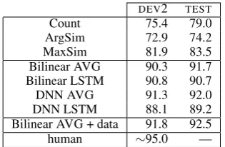
Final Results. Our final results are shown in
Ta-ble 5. We show theDEV2 andTESTaccuracies for
our baselines and for the best configuration (tuned onDEV2) for each model. All models outperform
all baselines handily. Our models perform simi-larly, with the Bilinear models and the DNN AVG model all exceeding 90% on bothDEV2 andTEST.
We note that the AVG models performed strongly compared to those that used LSTMs for
4These experiments were performed using 2 threads on a 3.40-GHz Intel Core i7-3770 CPU with 8 cores.
DEV2 TEST
Count 75.4 79.0
ArgSim 72.9 74.2
MaxSim 81.9 83.5
Bilinear AVG 90.3 91.7 Bilinear LSTM 90.8 90.7
DNN AVG 91.3 92.0
DNN LSTM 88.1 89.2
Bilinear AVG + data 91.8 92.5
[image:7.595.93.272.164.218.2]human ∼95.0 —
Table 5: Accuracies (%) of baselines and final model configurations onDEV2 andTEST. “+ data”
uses enlarged training set of size 300,000, and then doubles this training set by including tuples with conjugated forms; see text for details. Human per-formance onDEV2 was estimated from a sample
of size 100.
modeling terms. We suggest two reasons for this. The first is that most terms are short, with an aver-age term length of 2.3 words in our training tu-ples. An LSTM may not be needed to capture long-distance properties. The second reason may be due to hyperparameter tuning. Recall that we used a greedy search for optimal hyperparameter values; we found that models with LSTMs take more time per epoch, more epochs to converge, and exhibit more hyperparameter sensitivity com-pared to models based on averaging. This may have contributed to inferior hyperparameter values for the LSTM models.
We also trained the Bilinear AVG model on a larger training set (row labeled “Bilinear AVG + data”). We note that the ConceptNet tuples typ-ically contain unconjugated forms; we sought to use both conjugated and unconjugated words. We began with a larger training set of 300,000 tuples from ConceptNet, then augmented them to include conjugated word forms as in the following exam-ple. For the tuplehsoak in a hotspring, CAUSES,
get pruny skiniobtained from the OMCS sentence “The effect of [soaking in a hotspring] is [get-ting pruny skin]”, we generated an additional tuple hsoaking in a hotspring, CAUSES, getting pruny
skini. We thus created twice as many training tu-ples. The results with this larger training set im-proved from 91.7 to 92.5 on the test set. We re-lease this final model to the research community.
Bilinear AVG Bilinear LSTM DNN AVG DNN LSTM
CE hinge CE hinge CE hinge CE hinge
random 90 84 91 83 91 87 88 57
mix 90 83 90 87 90 78 82 63
[image:8.595.155.443.61.114.2]max 86 75 65 66 61 52 56 52
Table 3: Accuracies (%) on DEV2 of models trained with two loss functions (cross entropy (CE) and
hinge) and three sampling strategies (random, mix, and max). The best accuracy for each model is shown in bold. Cross entropy with random sampling is best across models and is also fastest (see Table 4).
queries. Our models are parametric models that can compress a large training set into a fixed num-ber of parameters. This makes them extremely fast for answering queries, particularly the AVG mod-els, enabling use in downstream NLP applications. 7 Generating and Scoring Novel Tuples We now measure our model’s ability to score novel tuples generated automatically from ConceptNet and Wikipedia. We first describe simple pro-cedures to generate candidate tuples from these two datasets. We then score the tuples using our MaxSim baseline and the trained Bilinear AVG model.5 We evaluate the highly-scoring tuples
us-ing a small-scale manual evaluation.
The DNN AVG and Bilinear AVG models reached the highestTESTaccuracies in our
evalua-tion, though in preliminary experiments we found that the Bilinear AVG model appeared to perform better when scoring the novel tuples described be-low. We suspect this is because the DNN func-tion class has more flexibility than the bilinear one. When scoring novel tuples, many of which may be highly noisy, it appears that the constrained struc-ture of the Bilinear AVG model makes it more ro-bust to the noise.
7.1 Generating Tuples From ConceptNet
In order to get new tuples, we automatically mod-ify existing ConceptNet tuples. We take an exist-ing tuple and randomly change one of the three fields (t1,t2, orR), ensuring that the result is not a
tuple existing in ConceptNet. We then score these tuples using MaxSim and the Bilinear AVG model and analyze the results.
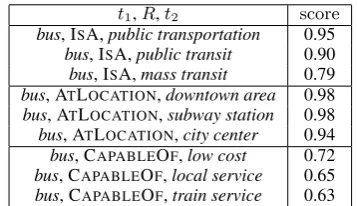
7.2 Generating Tuples from Wikipedia
We also propose a simple method to extract candi-date tuples from raw text. We first run the Stan-ford part-of-speech (POS) tagger (Toutanova et
5For the results in this section, we used the Bilinear AVG model that achieved 91.7 onTESTrather than the one aug-mented with additional data.
t1,R,t2 score
bus, ISA,public transportation 0.95 bus, ISA,public transit 0.90 bus, ISA,mass transit 0.79 bus, ATLOCATION,downtown area 0.98 bus, ATLOCATION,subway station 0.98 bus, ATLOCATION,city center 0.94 bus, CAPABLEOF,low cost 0.72 bus, CAPABLEOF,local service 0.65 bus, CAPABLEOF,train service 0.63 Table 6: Top Wikipedia tuples for 3 relations with
t1=bus, scored by Bilinear AVG model.
al., 2003) on the terms in our ConceptNet training tuples. We enumerate the 50 most frequent term pair tag sequences for each relation. We do lim-ited manual filtering of the frequent tag sequences, namely removing the sequences “DT NN NN” and “DT JJ NN” for the ISA relation. We do this in
or-der to reduce noise in the extracted tuples. To fo-cus on finding nontrivial tuples, for each relation we retain the top 15 POS tag sequences in which
t1ort2has at least two words.
We then run the tagger on sentences from En-glish Wikipedia. We extract word sequence pairs corresponding to the relation POS tag sequence pairs, requiring that there be a gap of at least one word between the two terms. We then remove word sequence pairs in which one term is solely one of the following words: be, the, always, there, has, due, however. We also remove tuples con-taining words that are not in the vocabulary of our ConceptNet-trained embeddings. We require that one term does not include the other term. We cre-ate tuples consisting of the two terms and all pos-sible relations that occur with the POS sequences of those two terms. Finally, we remove tuples that exactly match our ConceptNet training tuples.
[image:8.595.326.505.179.282.2]7.3 Manual Analysis of Novel Tuples
To evaluate our models on newly generated tu-ples, we rank them using different models and manually score the high-ranking tuples for qual-ity. We first randomly sampled 3000 tuples from each set of novel tuples. We do so due to the time requirements of the MaxSim baseline, which re-quires iterating through the entire training set for each candidate tuple. We score these sampled tu-ples using MaxSim and the Bilinear AVG model and rank them by their scores. The top 100 tu-ples under each ranking were given to an tor who is a native English speaker. The annota-tor assigned a quality score to each tuple, using the same 0-4 annotation scheme as Speer et al. (2010): 0 (“Doesn’t make sense”), 1 (“Not true”), 2 (“Opinion/Don’t know”), 3 (“Sometimes true”), and 4 (“Generally true”). We report the average quality score across each set of 100 tuples.
The results are shown in Table 7. To calibrate the scores, we also gave two samples of Concept-Net (CN) tuples to the annotator: a sample of 100 high-confidence tuples (first row) and a sample of 100 medium-confidence tuples (second row). We find the high-confidence tuples to be of high quality, recording an average of 3.68, though the medium-confidence tuples drop to 3.14.
The next two rows show the quality scores of the MaxSim baseline and the Bilinear AVG model. The latter outperforms the baseline and matches the quality of the medium-confidence ConceptNet tuples. Since our novel tuples are not contained in ConceptNet, this result suggests that our model can be used to add medium-confidence tuples to ConceptNet.
The novel Wikipedia tuples (top 100 tuples ranked by Bilinear AVG model) had a lower qual-ity score (2.78), but this is to be expected due to the difference in domain. Since Wikipedia con-tains a wide variety of text, we found the novel tuples to be noisier than those from ConceptNet. Still, we are encouraged that on average the tuples are judged to be close to “sometimes true.”
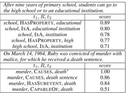
7.4 Text Analysis with Commonsense Tuples
We note that our method of tuple extraction and scoring could be used as an aid in applications that require sentence understanding. Two example sentences are shown in Table 8, along with the top tuples extracted and scored using our method. The tuples capture general knowledge about phrases
tuples quality
[image:9.595.315.518.60.125.2]high-confidence CN tuples 3.68 medium-confidence CN tuples 3.14 novel CN tuples, ranked by MaxSim 2.74 novel CN tuples, ranked by Bilinear AVG 3.20 novel Wiki tuples, ranked by Bilinear AVG 2.78
Table 7: Average quality scores from manual eval-uation of novel tuples. Each row corresponds to a different set of tuples. See text for details.
After nine years of primary school, students can go to the high school or to an educational institution.
t1,R,t2 score
school, HASPROPERTY,educational 0.89 school, ISA,educational institution 0.80 school, ISA,institution 0.78 school, HASPROPERTY,high 0.77 high school, ISA,institution 0.71 On March 14, 1964, Ruby was convicted of murder with malice, for which he received a death sentence.
t1,R,t2 score
murder, CAUSES,death∗ 1.00
murder, CAUSES,death sentence 0.86 murder, HASSUBEVENT,death 0.84 murder, CAPABLEOF,death 0.51
Table 8: Top ranked tuples extracted from two example sentences and scored by Bilinear AVG model.∗= contained in ConceptNet.
contained in the sentence, rather than necessarily indicating what the sentence means. This proce-dure could provide relevant commonsense knowl-edge for a downstream application that seeks to understand the sentence. We leave further investi-gation of this idea to future work.
8 Conclusion
We proposed methods to augment curated com-monsense resources using techniques from knowl-edge base completion. By scoring novel tuples, we showed how we can increase the applicability of the knowledge contained in ConceptNet. In fu-ture work, we will explore how to use our model to improve downstream NLP tasks, and consider applying our methods to other knowledge bases. We have released all of our resources—code, data, and trained models—to the research community.6
Acknowledgments
We thank the anonymous reviewers, John Wieting, and Luke Zettlemoyer.
6Available at http://ttic.uchicago.edu/
[image:9.595.310.524.182.340.2]References
Basant Agarwal, Namita Mittal, Pooja Bansal, and Sonal Garg. 2015. Sentiment analysis using common-sense and context information. Comp. Int. and Neurosc.
Gabor Angeli and Christopher Manning. 2013. Philosophers are mortal: Inferring the truth of un-seen facts. InProc. of CoNLL.
Gabor Angeli and D. Christopher Manning. 2014. NaturalLI: Natural logic inference for common sense reasoning. InProc. of EMNLP.
Collin F Baker, Charles J Fillmore, and John B Lowe. 1998. The Berkeley FrameNet project. InProc. of COLING.
Mohit Bansal, Kevin Gimpel, and Karen Livescu. 2014. Tailoring continuous word representations for dependency parsing. InProc. of ACL.
Kurt Bollacker, Colin Evans, Praveen Paritosh, Tim Sturge, and Jamie Taylor. 2008. Freebase: a col-laboratively created graph database for structuring human knowledge. InProc. of the ACM SIGMOD International Conference on Management of Data.
Antoine Bordes, Nicolas Usunier, Alberto Garcia-Duran, Jason Weston, and Oksana Yakhnenko. 2013. Translating embeddings for modeling multi-relational data. InAdvances in NIPS.
Antoine Bordes, Sumit Chopra, and Jason Weston. 2014a. Question answering with subgraph embed-dings. InProc. of EMNLP.
Antoine Bordes, Xavier Glorot, Jason Weston, and Yoshua Bengio. 2014b. A semantic matching en-ergy function for learning with multi-relational data.
Machine Learning, 94(2).
Erik Cambria, Daniel Olsher, and Kenneth Kwok. 2012. Sentic activation: A two-level affective com-mon sense reasoning framework. InProc. of AAAI.
Andrew Carlson, Justin Betteridge, Bryan Kisiel, Burr Settles, Estevam R Hruschka Jr, and Tom M Mitchell. 2010. Toward an architecture for never-ending language learning. InProc. of AAAI.
Luigi Di Caro, Alice Ruggeri, Loredana Cupi, and Guido Boella. 2015. Common-sense knowledge for natural language understanding: Experiments in unsupervised and supervised settings. In Proc. of AI*IA.
John Duchi, Elad Hazan, and Yoram Singer. 2011. Adaptive subgradient methods for online learning and stochastic optimization. JMLR.
Anthony Fader, Stephen Soderland, and Oren Etzioni. 2011. Identifying relations for open information ex-traction. InProc. of EMNLP.
Alberto Garc´ıa-Dur´an, Antoine Bordes, and Nicolas Usunier. 2014. Effective blending of two and three-way interactions for modeling multi-relational data. In Machine Learning and Knowledge Discovery in Databases.
Matt Gardner, Partha Pratim Talukdar, Jayant Krish-namurthy, and Tom Mitchell. 2014. Incorporat-ing vector space similarity in random walk inference over knowledge bases. InProc. of EMNLP. Jonathan Gordon and Lenhart K Schubert. 2012.
Using textual patterns to learn expected event fre-quencies. In Proc. of Joint Workshop on Auto-matic Knowledge Base Construction and Web-scale Knowledge Extraction.
Jonathan Gordon and Benjamin Van Durme. 2013. Reporting bias and knowledge acquisition. InProc. of Workshop on Automated Knowledge Base Con-struction.
Jonathan Gordon, Benjamin Van Durme, and Lenhart K Schubert. 2010. Learning from the web: Extracting general world knowledge from noisy text. In Collaboratively-Built Knowledge Sources and AI.
Jonathan Gordon. 2014. Inferential Commonsense Knowledge from Text. Ph.D. thesis, University of Rochester.
Kelvin Gu, John Miller, and Percy Liang. 2015. Traversing knowledge graphs in vector space. In
Proc. of EMNLP.
Felix Hill, Roi Reichart, and Anna Korhonen. 2015. SimLex-999: Evaluating semantic models with (genuine) similarity estimation.Computational Lin-guistics.
Sepp Hochreiter and J¨urgen Schmidhuber. 1997. Long short-term memory.Neural computation.
Po-Sen Huang, Xiaodong He, Jianfeng Gao, Li Deng, Alex Acero, and Larry Heck. 2013. Learning deep structured semantic models for web search using clickthrough data. InProc. of CIKM.
Rodolphe Jenatton, Nicolas L. Roux, Antoine Bordes, and Guillaume R Obozinski. 2012. A latent factor model for highly multi-relational data. InAdvances in NIPS.
Dan Klein and Christopher D. Manning. 2003. Accu-rate unlexicalized parsing. InProc. of ACL.
Ni Lao, Tom Mitchell, and William W Cohen. 2011. Random walk inference and learning in a large scale knowledge base. InProc. of EMNLP.
Douglas B Lenat and Ramanathan V Guha. 1989.
Henry Lieberman, Alexander Faaborg, Waseem Daher, and Jos´e Espinosa. 2005. How to wreck a nice beach you sing calm incense. InProc. of IUI.
Wang Ling, Chris Dyer, Alan W Black, Isabel Tran-coso, Ramon Fermandez, Silvio Amir, Luis Marujo, and Tiago Luis. 2015. Finding function in form: Compositional character models for open vocabu-lary word representation. InProc. of EMNLP.
Tomas Mikolov, Ilya Sutskever, Kai Chen, Greg S Cor-rado, and Jeff Dean. 2013. Distributed representa-tions of words and phrases and their compositional-ity. InAdvances in NIPS.
George A Miller. 1995. WordNet: a lexical database for English.Communications of the ACM, 38(11).
Mike Mintz, Steven Bills, Rion Snow, and Daniel Ju-rafsky. 2009. Distant supervision for relation ex-traction without labeled data. InProc of ACL.
Arvind Neelakantan and Ming-Wei Chang. 2015. In-ferring missing entity type instances for knowledge base completion: New dataset and methods. In
Proc. of NAACL.
Arvind Neelakantan, Benjamin Roth, and Andrew Mc-Callum. 2015. Compositional vector space models for knowledge base completion. InProc. of ACL.
Maximilian Nickel, Volker Tresp, and Hans-Peter Kriegel. 2011. A three-way model for collective learning on multi-relational data. InProc. of ICML.
Maximilian Nickel, Volker Tresp, and Hans-Peter Kriegel. 2012. Factorizing YAGO: Scalable ma-chine learning for linked data. InProc. of WWW.
Jeffrey Pennington, Richard Socher, and Christo-pher D. Manning. 2014. GloVe: Global vectors for word representation. InProc. of EMNLP.
Sebastian Riedel, Limin Yao, Andrew McCallum, and M. Benjamin Marlin. 2013. Relation extraction with matrix factorization and universal schemas. In
Proc. of NAACL-HLT.
Richard Socher, Danqi Chen, Christopher D Manning, and Andrew Ng. 2013. Reasoning with neural ten-sor networks for knowledge base completion. In Ad-vances in NIPS.
Robert Speer and Catherine Havasi. 2012. Represent-ing general relational knowledge in ConceptNet 5. InProc. of LREC.
Robert Speer, Catherine Havasi, and Henry Lieberman. 2008. AnalogySpace: Reducing the dimensionality of common sense knowledge. InProc. of AAAI.
Robert Speer, Catherine Havasi, and Harshit Surana. 2010. Using verbosity: Common sense data from games with a purpose. InProc. of FLAIRS.
Kristina Toutanova, Dan Klein, Christopher D Man-ning, and Yoram Singer. 2003. Feature-rich part-of-speech tagging with a cyclic dependency network. InProc. of NAACL-HLT.
Kristina Toutanova, Danqi Chen, Patrick Pantel, Hoi-fung Poon, Pallavi Choudhury, and Michael Gamon. 2015. Representing text for joint embedding of text and knowledge bases. InProc. of EMNLP.
Luis von Ahn, Mihir Kedia, and Manuel Blum. 2006. Verbosity: a game for collecting common-sense facts. InProc. of CHI.
Robert West, Evgeniy Gabrilovich, Kevin Murphy, Shaohua Sun, Rahul Gupta, and Dekang Lin. 2014. Knowledge base completion via search-based ques-tion answering. InProc. of WWW.
John Wieting, Mohit Bansal, Kevin Gimpel, Karen Livescu, and Dan Roth. 2015. From paraphrase database to compositional paraphrase model and back. Transactions of the ACL.
John Wieting, Mohit Bansal, Kevin Gimpel, and Karen Livescu. 2016. Towards universal paraphrastic sen-tence embeddings. InProc. of ICLR.
Bishan Yang, Wen-tau Yih, Xiaodong He, Jianfeng Gao, and Li Deng. 2014. Embedding entities and relations for learning and inference in knowledge bases. arXiv preprint arXiv:1412.6575.