Munich Personal RePEc Archive
The impact of oil and gold price
fluctuations on the South African equity
market: volatility spillovers and
implications for portfolio management
Morema, Kgotso and Bonga-Bonga, Lumengo
University of Johannesburg, University of Johannesburg
10 April 2018
Online at
https://mpra.ub.uni-muenchen.de/87637/
THE IMPACT OF OIL AND GOLD PRICE FLUCTUATIONS ON THE SOUTH
AFRICAN EQUITY MARKET: VOLATILITY SPILLOVERS AND IMPLICATIONS
FOR PORTFOLIO MANAGEMENT
BY
KGOTSO MOREMA
AND
LUMENGO BONGA-BONGA
ABSTRACT
This paper aims to study the impact of gold and oil price fluctuations on the volatility of the
South African stock market and its component indices or sectors – namely, the financial,
industrial and resource sectors – making use of the asymmetric dynamic conditional correlation
(ADCC) generalised autoregressive conditional heteroskedasticity (GARCH) model. Moreover,
the study assesses the magnitude of the optimal portfolio weight, hedge ratio and hedge
effectiveness for portfolios that are constituted of a pair of assets, namely oil-stock and
gold-stock pairs. The findings of the study show that there is significant volatility spillover between
the gold and the stock markets, and the oil and stock markets. This finding suggests the
importance of the link between futures commodity markets and the stock markets, which is
essential for portfolio management. With reference to portfolio optimisation and the possibility
of hedging when using the pairs of assets under study, the findings suggest the importance of
combining oil and stocks as well as gold and stocks for effective hedging against any risks.
Keywords: Hedge ratio, optimal portfolio weight, ADCC model, crises, hedge effectiveness,
1. INTRODUCTION
Over the past years, the South African stock market has shown significant growth, with market
capitalisation increasing from 545.4 billion dollars in 2005 to 612.3 billion in 2012 and the
turnover ratio increasing by 15.6 percentage points during the period 2005 to 2012
(https://data.worldbank.org). This growth has attracted a number of domestic and international
investors in search of high yields (Zhang, Li & Yu, 2013).
However, despite their high yields, emerging markets, such as that of South Africa, are known to
be vulnerable to shocks from developed markets. A number of studies indicate how emerging
markets have been exposed to the different crises, such as: the dot-com bubble crisis from 2000
to 2001; the global financial crisis from 2007 to 2008; and the European debt crisis from 2010 to
2011 (see Heymans & da Camara, 2013). This vulnerability of emerging markets to external
shocks has been a concern to policy makers, investors and asset managers, who seek different
ways to minimise the risk thereof. For example, asset managers in search of high yields in
emerging stock markets often seek effective methods to minimise risk exposure in these markets.
Literature suggests a number of ways to hedge risk exposure in stock markets. For example,
Chkili (2016) and Khalfaoui, Boutahar and Boubaker (2015) find that investment in oil and gold
markets provides an opportunity to hedge against stock market exposure in developed
economies. However, to the best of our knowledge, there is a deficit in the literature that seeks to
assess the link among gold, oil and stock markets in the context of emerging market economies,
especially for South Africa. Since South Africa is a net oil-importing and net gold-exporting
country, there is no doubt that the country may be exposed to shocks in the gold and oil prices. In
addition, assessing the extent of shock transmission and the relation between stock markets and
commodity (oil and gold) prices should provide insight into how investors’ positions can be
combined when making hedging decisions (Ewing & Malik, 2013).
There is a significant number of studies which assessed the impact of oil prices on stock market
prices in other countries. For example, Huang, Masulis and Stoll (1996) found that higher oil
prices result in changes in a country’s trade balance and current account, which, in turn, affect
(1999), Anoruo and Mustafa (2007), and Park and Ratti (2008) examined the relationship
between oil and the stock market returns in the United States of America (US), finding that oil
price fluctuations have a negative effect on stock returns in this country. In contrast, Cong, Wei,
Jiao and Fan (2008) concluded that there isn’t any significant evidence on the relation between
oil price volatility and stock returns in China.
Other studies have assessed whether oil market can be a useful tool for hedging against stock
market exposure. For example, Chkili, Aloui and Nguyen (2014) studied the volatility
transmission and hedging strategies between US stock markets and crude oil prices. The authors
concluded that investors who seek to minimise portfolio risk should include oil and stock assets.
Similar studies – by Ewing and Malik (2016), Sadorsky (2012), Sadorsky (2014b), Arouri, Jouini
and Nguyen (2012) and Lin, Wesseh Jr. and Appiah (2014) – also find that oil is an effective
hedge for stock market exposure.
With regards to the link between gold and stock markets, Coudert and Raymond-Feingold (2011)
show that, during periods of crises, stock prices are most likely to drop and investors tend to
invest in safer assets, such as gold. Thus, it is expected that the gold market and stock market
will co-move, and the combination of instruments within the two markets should provide the best
opportunity for hedging. Also relevant are the findings by Baur and Lucey (2010), who examine
the constant and dynamic relationship between the stock markets, bonds and gold returns in the
US, United Kingdom and Germany, and explore whether gold plays a hedging role against stock
market exposure and safe haven during financial crises. The authors conclude that gold can be a
useful hedging tool as well as a safe haven against stock market exposure. Similar studies
conducted by Hood and Malik (2013) and Ciner, Gurdgiev and Lucey (2013) also suggest that
gold has the characteristic of being a good hedge against stock market exposure.
Indeed, there are many studies in developed markets that have studied the role of gold and oil in
portfolio diversification and hedging. However, as stated above, there is not enough literature
focusing on emerging markets. Among such existing studies is that by Basher and Sadorsky
(2016), which assesses the extent of volatility spillovers of oil, gold, volatility index (VIX) and
bonds in emerging stock markets (including South Africa), and compares the hedge effectiveness
of oil, gold, VIX and bonds against stock market exposure. Their findings show that oil provides
This paper will extend the study by Basher and Sadorsky by assessing the extent of volatility
spillover and the possibility of portfolio selection and hedging between the oil, gold and stock
markets at a disaggregated or sectoral level rather than at an aggregate level. Indeed, one of the
aims of this paper will be to assess the extent of volatility spillover between oil returns and the
returns of the resources sector rather than all stock market returns. In so doing, this paper will
depart from the past empirical studies that were focused on an aggregate regional,
country-specific or global stock market level, such as in Bhar and Nikolova (2009), Hammoudeh, Sari,
Uzunkaya and Liu (2013) and Xu and Hamori (2012).
Thus, the purpose of this study is to investigate the correlation and volatility spillovers between
oil, gold, and sectoral stock markets by making use of an asymmetric dynamic conditional
correlation model (ADCC) of Cappiello, Engle and Shepparad (2006). Moreover, the paper will
assess the possibility of optimal portfolio selection and hedging when combining assets from
each of the three markets.
The contribution of this paper is threefold. Firstly, instead of focusing only on the impact of gold
and oil volatility shocks on the aggregate stock market, as Basher and Sadorsky (2016) did, this
study will analyse volatility spillovers between gold, oil and the South African stock market at an
aggregated and disaggregated level. Secondly, we will analyse the optimal weights, hedge ratios
and effective portfolio weight for pairs of stock-oil and stock-gold portfolios. Lastly, this paper
will assess which of the commodities – oil or gold – provides a better hedge against stock market
exposure. Our research provides beneficial and extensive information to portfolio managers and
investors based on the interaction between the markets under study in the context of South
Africa. Furthermore, this study may also serve as a reference for investors, policy makers,
portfolio managers and researchers in terms of developing better and more effective trading
strategies.
The remainder of this paper is organized as follows; Section 2 provides a review on previous
theoretical and empirical literature related to this paper. Section 3 explains the theoretical
framework of econometric models which are used in the paper. Section 4 will discuss the process
of data collection and empirical results by applying and testing the models discussed in the
previous section (section 3). Lastly section 5 will conclude the paper by highlighting and
2. LITERATURE REVIEW
This section will focus on examining empirical and theoretical relationships of stock, oil and gold
prices.In a pioneering study, Chen, Roll and Ross (1986) explores different economic forces
(including oil) which are likely to influence the stock market using ordinary least squares. The
paper concludes that oil prices are a risk factor for stock price. Following this study, there has been
numerous studies on the relationship between the stock market and oil prices. For example, Jones
and Kaul (1996) investigate the effect of oil price shocks to the stock markets in Canada, Japan,
United Kingdom and USA using a cash-flow dividend valuation model. The paper concludes that
oil shocks have a negative significant effect on stock prices (except for UK).
Sadorsky (1999) examined the dynamic relationship between oil price, stock returns and a number
of economic variables in USA. The author makes use of an unrestricted vector auto-regression and
concluded that oil price shocks have a negatively significant effect on stock returns. Using a
standard market model augmented by oil price factor, Nandha and Faff (2008) investigate the
effect of oil price shocks on 35 DataStream global industry indices for the period between 1983
and 2005. The paper show evidence of significant negative impact of oil shocks on all industries’
equity returns.
Chiou and Lee (2009) used an Autoregressive Conditional Jump Intensity to study the relationship
between oil price shocks and the S&P500 index. The authors find that oil price shocks have a
negative impact on S&P500 index. Chiou and Lee also conclude that there are negative asymmetric
effects between oil price shocks and S&P500 returns during periods of high oil price volatility.
Similar studies by Malik and Ewing (2009), and Sadorsky (2008) also researched on the
relationship between the stock exchange market and oil market, and show that there exists a
negative correlation between the two markets.
On the contrary, there is a set of studies that argue that there exists a positive relationship between
oil prices and the stock market. For example, Basher and Sadorsky (2006) study the linkage
between oil price shocks and 21 emerging stock market returns using an international multi-factor
model which permits for both conditional and unconditional risk factors. The study show that in
Brailsford (1999) research the link between Australian stock market and oil prices using. They
found that the stock market has a positive correlation between oil and gas.
Narayan and Narayan (2010) also study the relationship between oil price and stock market in
Vietnam by using Gregory and Hansen residual based test. The paper conclude that in the
long-run oil price and exchange rate have positive significantly effects on the stock price. In addition,
Al-Mudhaf and Goodwin (1993), Sadorsky (2001) and Aloui, Hammoudeh, and Nguyen (2013)
also support the argument that oil prices and stock market prices are positively correlated.
However, there are also studies which provide evidence that the oil market has no impact on the
stock exchange market. Apergis and Miller (2009) investigate the impact of oil market shocks on
eight developed countries’ stock markets using a VEC model. The authors find that there is no
significant relationship between oil market and the stock market. Furthermore, Hung et al. (1996)
also examined the relation between oil future prices and the S&P 500 and found that it is
non-existent. The paper used a VAR approach to reach this conclusion. Similar findings are given by
Chen et al. (1986), and Lescaroux and Mignon (2008).
Moreover, there is also work which investigates the volatility transmission of oil and the stock
market, and the role of oil as a hedging instrument. Kilian and Park (2009) explained that the
relationship between oil prices and the stock market can either be positive or negative depending
on whether the shock in oil price is driven by demand or supply shocks in the oil market. Therefore,
it is important to differentiate between oil-exporting countries and non-oil-exporting countries
when investigating this relationship.
On the other hand, there is not much literature on the relationship between gold and the stock
market; most studies focus more on the role of gold as a hedge or safe haven. Among studies,
Hood and Malik (2013) assess the role of gold, other precious metals and volatility index (VIX)
as a hedge and safe haven for the stock market in USA. Using a regression model by Baur and
McDermott (2010), the authors conclude that gold serves as a better hedge and safe haven than
other precious metals. However VIX serves as a better hedge and safe haven than gold. Similarly,
Baur and Lucey (2010) and Ciner, Gurdgiev and Lucey (2013) also suggest that gold has
Equally important, there are also studies which investigate the volatility spillovers between gold
and the stock market, and the role of gold as a hedge instrument. For example, Arouri, Lahiani,
Nguyen (2015) investigate the volatility spillovers between the Chinese stock market prices and
gold prices using the VAR-GARCH. The paper suggest that there are volatility spillovers between
china’s change in stock prices and gold price, and adding gold in a stock portfolio can help
minimize stock market risk.
Ewing and Malik (2013) stated that there is strong evidence of volatility spillovers between the
gold and stock market. The paper used univariate and bivariate GARCH models to achieve such
results. Kumar (2014) study the volatility spillovers between gold and sector stock returns, and the
role of gold as a hedge using a generalised VAR-ADCC-BVGARCH model. The study show that
the correlation varies over time and during periods of crisis, therefore, including gold in a portfolio
provides an effective hedged portfolio. Furthermore, Chkili (2016) used an ADCC-GARCH
model, respectively, to study the relation between gold and the stock market. They find correlation
to vary over time and suggest that gold is a good hedge and it can also play a role of a safe haven
during periods of crises. A similar studies by Gurgun and Unalmis¸ (2014) also suggest that gold
is a good hedge and safe haven.
The above studies are among the small body of literature on the relationship between oil, gold and
stock prices. The Studies show the relationship of oil, gold and the stock prices, and the role of
oil and gold as hedge instruments for the stock market. However, there are few studies which are
focused on the relationship between oil, gold and stock prices in African countries. For example,
Basher and Sadorsky (2016) investigates the effectiveness of oil, gold, bonds and VIX as hedge
instruments for emerging market stocks, using a DCC, ADCC and GO-GARCH to estimate
conditional volatilities and correlations. The paper concludes that both oil and gold can be used as
hedge instruments, but oil provides a more effective hedge than gold. However, this study fails to
provide the role of oil and gold as a hedge for different stock sectors. Contrary to the study by
Basher and Sadorsky (2016), this paper will contribute to the literature of the volatility spillovers
between oil, gold and stock prices, by evaluating volatility spillovers between oil, gold and seven
most volatile stock market sectors in South Africa. Moreover, this paper will advise investors on
3. METHODOLOGY
This section explains the methodology used in this study, and it is presented as follows. To begin
with, we will explain how to model time varying volatility and correlations among the variables
under study. Followed by, an analysis of optimal portfolio weights. Then, we give details on how
to compute optimal hedge ratios. To finish, we provide an assessment of hedge effectiveness.
This paper will adopt an asymmetric dynamic conditional correlation model of Cappiello, Engle
and Shepparad (2006) to model conditional volatility, correlations, optimal weights and hedge
ratios for oil-stock and gold-stock pairs. Recent literature shows that an ADCC model is by far the
best model to estimate conditional correlation, variances and covariances among time series
because it accounts for both the dynamic correlation and the asymmetric feature of stock market’s
behavior (Ederington and Guan, 2010, and Chkili, 2016).
3.1Asymmetric Dynamic Conditional Correlation Model
The ADCC formulated by Cappiello et al. (2006) follows a two-step estimation process. The first
step is to estimate the conditional variances. To do so, we first need to obtain random error terms
from the conditional mean model. We will use a VAR model as it permits for autocorrelations and
cross-autocorrelations in returns.
𝑟𝑖𝑡 = 𝐶𝑖 + ∑𝑛𝑗=1𝜔𝑖𝑗𝑟𝑖𝑡−1+ 𝜀𝑖𝑡 , 𝜀𝑖𝑡|𝐹𝑡−1 ~ 𝑁(0 , ℎ𝑖𝑖𝑡) (9)
𝜀𝑖𝑡 = 𝑒𝑖𝑡√ℎ𝑖𝑖𝑡 , 𝑒𝑖𝑡~ 𝑁(0 , 1) (10)
where equation (9) represents the mean equation given as a VAR model with one lag. 𝑟𝑖𝑡is a 1xn
vector of daily returns of oil, gold and major sectors mentioned in the previous section, and it is
calculated as 𝑟𝑖𝑡 = log ( 𝑃𝑖𝑡
𝑃𝑖𝑡−1) ∗ 100, where 𝑃𝑖𝑡 is the closing price of 𝑖 at time 𝑡. 𝐶 𝑖 is the
long-term drift coefficient for variable 𝑖. The parameter 𝜔𝑖𝑗 for 𝑖 = 𝑗 indicates the effect of previous 𝑖
returns of 𝑖. 𝐹𝑡−1 is the market information available at time t − 1. Lastly, 𝜀𝑖𝑡 represents the random
error term for variable 𝑖 at time 𝑡.
Equation (10) shows 𝜀𝑖𝑡(error terms), and 𝑒𝑖𝑡 represents standardised residuals, which follows
a joint normal distribution.
This paper will use the VARMA-GARCH (1, 1) developed by Ling and McAleer (2003) to
model conditional variances and covariances. This method is useful when modeling volatility
spillovers, because unlike a simple GARCH (1, 1) model, a VARMA-GARCH (1,1) has the
ability to show how shocks in one variable can affect the variances of the other variables
(Sadorsky, 2012). A VARMA-GARCH (1, 1) is specified as follows:
ℎ𝑖𝑖𝑡 = 𝜑𝑖 + ∑𝑛𝑗=1𝛼𝑖𝑗𝜀2𝑖𝑡−1+ ∑𝑛𝑖=1𝛾𝑖𝜀2𝑖𝑡−1𝐷𝑖𝑡−1+ ∑𝑛𝑗=1𝛽𝑖𝑗ℎ𝑖𝑡−1 (11)
where ℎ𝑖𝑖𝑡is the conditional variance, 𝜑𝑖 denotes the constant term of the conditional variance
equations for 𝑖. ∑𝑛𝑗=1𝛼𝑖𝑗 for 𝑖 = 𝑗 denotes 𝑖′s own ARCH effect, which measures the
short-run volatility persistence. ∑𝑛𝑗=1𝛽𝑖𝑗 for 𝑖 = 𝑗 denotes 𝑖′𝑠 own GARCH terms, which measure
the long-run volatility persistence. For 𝑖 ≠ 𝑗, ∑𝑛𝑗=1𝛼𝑖𝑗 and ∑𝑛𝑗=1𝛽𝑖𝑗 respectively denote the
cross ARCH and GARCH terms, which measure the volatility spillovers from 𝑗
to 𝑖. 𝛾𝑖𝜀2𝑖𝑡−1𝐷𝑖𝑡−1 captures leverage effects (asymmetry), where 𝐷𝑖𝑡−1 is a dummy variable
and equals one when 𝜀2𝑖𝑡−1 < 0 and 0 otherwise. The term 𝐷𝑖𝑡−1 allows bad news in the
market (𝜀2𝑖𝑡−1 < 0) to be followed by higher volatilities than good news (𝜀2𝑖𝑡−1 > 0) of the
same magnitude.
In the second step, we estimate conditional correlations based on the standardised residuals
from step one, as follows:
𝐻𝑡 = 𝐷𝑡𝑃𝑡𝐷𝑡 (12)
where 𝐻𝑡 is an nxn conditional covariance matrix, 𝐷𝑡 is a diagonal matrix with conditional
𝑃𝑡 =
[ 1
√𝑞11𝑡 0 ⋯ 0
0
⋮ ⋱ 0⋮
0 0 ⋯ √𝑞1
𝑛𝑛𝑡]
∗ 𝑄𝑡∗
[ 1
√𝑞11𝑡 0 ⋯ 0
0 ⋱ 0⋮
0 0 ⋯ √𝑞1
𝑛𝑛𝑡]
(15)
𝑄𝑖𝑗𝑡 = (1 − 𝑓1− 𝑓2)𝑄̅ + 𝑓1𝑢𝑖𝑡−1𝑢′𝑗𝑡−1+ 𝑓2𝑄𝑖𝑗𝑡−1 (16)
where 𝑄𝑖𝑗𝑡 is the unconditional variance between 𝑖 and 𝑗, and is a positive definite nxn
matrix. 𝑄 ̅̅̅̅ a is an nxn unconditional covariance matrix, 𝑢𝑡−1 represents standardised residuals
and 𝑓1 and 𝑓2are non-negative parameters, where 𝑓1+ 𝑓2 < 1. The time-varying conditional
correlation coefficient is expressed as:
𝜌𝑖𝑗𝑡 =√𝑞𝑞𝑖𝑖𝑡𝑖𝑗𝑡𝑞𝑗𝑗𝑡 (17)
An asymmetric DCC model will be estimated using a Quasi-Maximum Likelihood Estimation
(QMLE) with the Broyden-Fletcher-Goldfarb-Shanno (BFGS) algorithm and the T statistics
being computed by a robust estimate of the covariance matrix.
4.3.2 Optimal Portfolio Weights
To construct an optimal portfolio that minimizes risk without lowering expected returns, we use a
methodology by Kroner and Ng (1998) to construct optimal portfolio weights of a two asset
portfolio as follows:
𝑤𝑆𝑂,𝑡 =ℎ ℎ𝑖,𝑡−ℎ𝑖𝑗,𝑡
𝑗,𝑡−2ℎ𝑖𝑗,𝑡+ℎ𝑖,𝑡 (11)
, and
𝑤𝑆𝑂,𝑡 = {
0, 𝑖𝑓 𝑤𝑖𝑗,𝑡 < 0 𝑤𝑖𝑗,𝑡, 𝑖𝑓 0 ≤ 𝑤𝑖𝑗,𝑡 ≤ 1
1, 𝑖𝑓 𝑤𝑖𝑗,𝑡 > 1
(12)
Where 𝑤𝑖𝑗,𝑡 refers to the weight of 𝑗 in a portfolio of the two assets defined above at time 𝑡 and
weight of 𝑗 in the considered portfolio is obtained by (1 − 𝑤𝑖𝑗,𝑡).
Alternatively, in order to minimize risk we will follow Kroner and Sultan (1993) regarding risk
minimizing hedge ratios of a two-asset portfolio. We typically seek the amount of the short position
taken in 𝑗 in order to minimize the risk of a long position in 𝑖. The optimal hedge ratio is as follows:
𝛽𝑖𝑗,𝑡 =ℎℎ𝑖𝑗,𝑡𝑖,𝑡 (13)
Where 𝛽𝑖𝑗,𝑡represents the optimal hedge ratio, ℎ𝑖,𝑡and ℎ𝑗,𝑡is the conditional variance of asset 𝑖,
conditional variance of asset 𝑗, respectively. ℎ𝑖𝑗,𝑡 denotes the conditional covariance of asset 𝑖
and 𝑗.
3.3.4 Measuring the Performance of a Hedged Portfolio
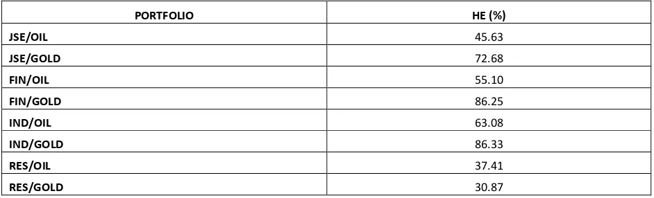
Most studies use the hedge effectiveness index given by Ederington (1979) to analyse the
performance of a hedged portfolio (Chkili, 2016 and Basher & Sadorsky, 2016). We will also
apply this hedge effectiveness index in our analysis below. The hedge effectiveness index is a
comparison of risk between a hedged and an un-hedged portfolio. A hedged portfolio comprises a
long position in the underlying stock and a short position in futures’ contracts. An unhedged
portfolio consists of only a long position in the underlying stock.
A hedge effectiveness index computes the percentage of the variance that is eliminated from an
unhedged portfolio by hedging, and is calculated as follows:
𝐻𝐸 =𝑉𝑎𝑟𝑖𝑎𝑛𝑐𝑒𝑈−𝑉𝑎𝑟𝑖𝑎𝑛𝑐𝑒𝐻
𝑉𝑎𝑟𝑖𝑎𝑛𝑐𝑒𝑈 (22)
Where 𝑉𝑎𝑟𝑖𝑎𝑛𝑐𝑒𝐻 and 𝑉𝑎𝑟𝑖𝑎𝑛𝑐𝑒𝑈 denote hedged and unhedged variances respectively.
This method compares the variance of the hedged portfolio to that of an un-hedged portfolio.
Hence, a higher hedge effectiveness (𝐻𝐸) implies that a higher variance (risk) is eliminated by the
4. DATA, ESTIMATION AND DISCUSSION OF RESULTS 4.1Data
The data used in this paper includes daily closing values of: FTSE/JSE All Share Index (JSE),
FTSE/JSE Financials (FIN), FTSE/JSE Industrials Index (IND), FTSE/JSE Resources (RES),
nearby futures’ contract of gold (GOLD) and nearby futures’ contract of Brent crude oil (OIL).1
All prices are expressed in US dollars.2 The sample period starts from 3 January 2006 and ends on
31 December 2015, taking into account both the global financial crisis and the European debt
crisis. We make use of daily data in order to capture the intensity and speed of the dynamic
transmission between commodity and stock markets’ returns. Data on FTSE/JSE indices is
obtained from Inet BFA, while OIL and GOLD data is from Bloomberg. In total, our analysis
includes 2581 observations. The sector indices included in this study are weighted by market
capitalisation, and they contain a bulk of stocks within their respective economic groups. We thus
assume that they can accurately display the aggregate stock price movements of firms within their
respective sectors.
Figure 1 below illustrates the returns of JSE, FIN, IND, RES, GOLD and OIL. Looking figure 1,
there is clear evidence of volatility clustering for all variables, with a noticeable high spike in 2007
- 2009, which is the result of the global financial crisis of 2008. Moreover, the high volatility
clustering from 2010 to 2011 should be attributed to the European debt crisis. OIL also shows high
volatility clustering in 2014 to 2015, which could reflect the effects of the oil price crisis. Lastly,
there is a spike in GOLD in 2013, which was due to global inflation falling in 2013, reducing the
value of gold as a hedge against inflation3.
Table 2 below represents the descriptive statistics of returns for all variables under study. All
time-series here indicate very similar descriptive statistics, especially for the means of the variables. For
example, the mean and median values are very close to zero and the unconditional standard
deviation is greater than the mean value for all variables. The standard deviation of OIL and RES
is greater than the standard deviations of all other variables, which is an indication that OIL and
1 Note: we use the futures contract of gold and oil and not their spot prices, because the basic concept of hedging is to build a hedged portfolio
that will minimise risk by combining futures’ and spots’ positions. Therefore, since this paper aims to analyse the hedge effectiveness of oil and gold against stock market exposure, using future prices will be more appropriate to determine optimal hedge ratios.
RES are more volatile than the other variables in the study. The least volatile series is IND, with a
standard deviation of 1.0838. The skewness and kurtosis for all variables show that the returns are
not normally distributed, confirmed by the Jarque-Bera normality test, which is typical for
financial time-series behaviour.
Furthermore, we also calculate unconditional correlations of pairs of stock4-oil and stock-gold returns. Such correlations between returns are often used to guide portfolio diversification
decisions. However, unconditional correlations fail to account for the dynamic behaviour of
correlations between returns, which will be addressed below.5 The correlations for stock-oil pairs
are positive for all pairs, suggesting that, over our sample period, increases in oil prices were seen
as being indicative of higher earnings in the stock market. However, the correlations for
stock-gold pairs are weak and positive for all pairs, except for the RES and GOLD pair. The highest
correlation is that of OIL-RES (0.3518) and GOLD-RES (0.3281) pairs. This result is expected,
as the resources index includes stocks of companies involved in gold mining and oil exploration.
The lowest correlation is observed for the IND-GOLD pair (0.0688). Overall, the correlation of
returns between stock-oil and stock-gold pairs under study are relatively low, suggesting that there
might be an opportunity for meaningful portfolio diversification.
JSE FIN IND RES OIL GOLD
Mean 0.0394 0.0327 0.0627 -0.0094 -0.0193 0.0270
Median 0.0450 0.0248 0.0865 0.0000 0.0000 0.0375
Std. dev 1.2705 1.2579 1.0838 1.9309 2.1085 1.2655
Variance 1.6142 1.5824 1.1745 3.7282 4.4457 1.6015
Skewness -0.1807 -0.1527 -0.1347 -0.0390 -0.0682 -0.5195
Kurtosis 3.8021 3.9456 3.3906 4.1658 3.7725 4.8373
Jarque-Bera
(Probability)
1568.6927
(0.0000)
1684.2184
(0.0000)
1244.1261
(0.0000)
1866.8886
(0.0000)
1532.5127
(0.0000)
2632.4927
(0.0000)
Corr. With OIL 0.3240 0.2059 0.2340 0.3518 1.0000 0.2373
Corr. With GOLD 0.2216 0.0395 0.0688 0.3281 0.2373 1.0000
-4 -2 0 2 4
06 07 08 09 10 11 12 13 14 15
JSE -4 -2 0 2 4
06 07 08 09 10 11 12 13 14 15
FIN -3 -2 -1 0 1 2 3
06 07 08 09 10 11 12 13 14 15
IND -6 -4 -2 0 2 4 6
06 07 08 09 10 11 12 13 14 15
RES -6 -4 -2 0 2 4 6
06 07 08 09 10 11 12 13 14 15
OIL -6 -4 -2 0 2 4
06 07 08 09 10 11 12 13 14 15
GOLD
Note: the shaded area is the global financial crisis and the first and second phases of Eurozone sovereign debt crisis period (see table
[image:15.612.76.548.68.361.2]1 for more details).
Figure 1: JSE, FIN, IND, RES, GOLD and OIL Returns6
4.2Empirical Results7
4.2.1 The ADCC model estimation results from models 1 – 4
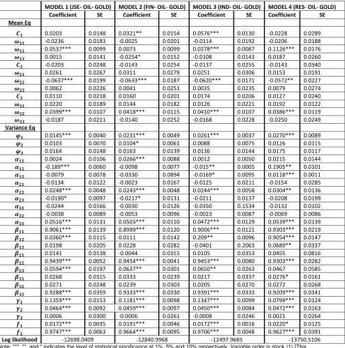
Table 4 shows the parameter obtained from the quasi-maximum likelihood estimation of equations
(9), (11), (12) and (16), representing the VAR-ADCC-GARCH model. Four models are estimated
combining three variables each: gold, oil and each of the three stock market sectors and the
aggregate stock market. For example, model 1 contains JSE (aggregate stock), OIL and GOLD;
model 2 contains FIN, OIL and GOLD; model 3 contains IND, OIL and GOLD; and model 4
contains RES, OIL and GOLD. To ensure accuracy, we will interpret the returns and volatility
spillover results for each model individually. The asymmetry and correlation coefficients results
will be interpreted jointly, as the outcomes are similar in all four models.
6 Unless specified otherwise, the shaded area in all graphs represents the global financial crisis and the first and second phases of the Eurozone
sovereign debt crisis.
7To ensure brevity, our interpretation below will we focus on OIL-STOCK and GOLD-STOCK pairs throughout the paper and not OIL-GOLD pairs.
Model 18
To study the volatility spillovers between the stock markets and commodity markets, it is necessary
to first identify the appropriate autoregressive model in order to determine the structure of the
volatility model that characterises each of the series. We will employ a VAR model of order 1
(VAR (1)) to model mean returns (equation 9). There are a number of reasons why we use a VAR
(1) process to model stock returns. Firstly, numerous recent empirical studies support the use of a
VAR (1) process for modelling stock market returns in emerging economies (for example, Chkili,
2016; Kang et al., 2016; Kumar, 2014; Basher & Sadorsky, 2016, etc.). Secondly, this model takes
into account the dynamics in market returns and indicates the speedy reaction of markets to new
information (Kumar, 2014). Thirdly, it captures the random walk and weak-form efficiency
characteristics of stock market prices and commodity prices (Fama, 1965). The same reasons apply
to the other three models below.
In table 4, model 1, the mean equation shows that own one period lagged JSE and GOLD returns,
denoted by the AR (1) coefficients (represented by 𝜔11 and 𝜔33 respectively) are not significant.
Thus past realisations of JSE and GOLD returns might not be useful in predicting future JSE and
GOLD returns respectively. In contrast, the AR (1) coefficient for OIL returns (represented by𝜔22)
is significant at a 1% level. This result suggests that past oil price changes can be used to predict
its own future returns. Moreover, the mean equation also shows cross returns spillovers
(cross-autocorrelations in returns) between the variables under study. We notice that there is a positive
significant return spillover from past OIL returns to current JSE returns (𝜔12). However, there is
no significant return spillover from past GOLD returns to the current JSE returns (𝜔13), implying
that current returns of JSE are significantly affected by past returns of OIL, and are unaffected by
past returns of GOLD. Furthermore, we do not find any significant return spillover from JSE
returns to both OIL (𝜔21) and GOLD returns (𝜔31), implying that past JSE returns might not be
useful when predicting future OIL or GOLD returns.
The next step when studying the volatility transmission between stock markets and commodity
markets involves the estimation of equations (11) and (12). From the variance equation (11) in
model 1 (see table 4), we obtain own ARCH (𝛼𝑖𝑖) and GARCH (𝛽𝑖𝑖) coefficients, which
respectively capture own volatility shock and own volatility persistence in the conditional variance
equations. For own ARCH coefficients, 𝛼11 refers to the ARCH term in the JSE equation, 𝛼22
refers to the ARCH term in the OIL equation and 𝛼33 refers to the ARCH term in the GOLD
equation. From our results in model 1, the estimated coefficients on own past volatility shocks
terms (denoted by 𝛼𝑖𝑖) are all significant at a 1% level in each equation, except for the JSE
equation, with 𝛼11 being insignificant. These results indicate that the current conditional volatility
of a specific variable (OIL and GOLD) depends on its own past volatility shocks, demonstrating
the importance of previous volatility shocks in explaining current conditional volatility.
Similarly, for own GARCH coefficients, 𝛽11 denotes the GARCH term in the JSE equation, 𝛽22
denotes the GARCH term in the OIL equation and 𝛽33 denotes the GARCH term in the GOLD
equation. From our results in model 1, it is evident that the estimated coefficients on own past
volatility persistence terms (denoted by 𝛽𝑖𝑖) are all statistically significant at a 1% level in each
equation. These results indicate that the current conditional volatility of a specific variable (JSE,
OIL and GOLD) depends on its own past volatility. This finding shows the importance of previous
volatility persistence in explaining current conditional volatility.
The results of model 1 also show that all ARCH parameters (𝛼𝑖𝑖) are relatively smaller than
GARCH parameters (𝛽𝑖𝑖), implying that the estimated conditional volatility does not swiftly
change, owing to a shift in volatility shocks (as shown by the small ARCH coefficients). Instead,
conditional volatility tends to gradually evolve over time with respect to large effects of past
volatility persistence (this result is similar in all cases under study). This finding will help investors
and portfolio managers to develop investment strategies that are focused on current market trends
and the long-run volatility persistence. Our results are very close to those of Sadorsky (2012) and
Kumar (2014).
In our analysis of the cross volatility transmission between OIL and JSE, and GOLD and JSE9 under model 1, the coefficients 𝛼𝑖𝑗 and 𝛽𝑖𝑗, where 𝑖 ≠ 𝑗, denote the short-run and long-run
persistence volatility transmission between stock and commodity markets under study
respectively. Our coefficients of interest in this case are;
9 Note: we focus on OIL-STOCK and GOLD-STOCK pairs throughout the paper and not OIL-GOLD pairs because the
𝛼12, which captures the short-run volatility shock from OIL to the stock (JSE in model 1,
FIN in model 2, IND in model 3 and RES in model 4), and 𝛽12, which measures the
long-run volatility persistence from OIL to the stock.
𝛼21, which captures the short-run volatility shock from the stock to OIL, while 𝛽21
measures the short-run volatility persistence from the stock to OIL.
𝛼13, which captures the short-run volatility shock from GOLD to the stock, and 𝛽13, which
measures the long-run volatility persistence from GOLD to the stock.
𝛼31, which captures the short-run volatility shock from the stock to GOLD, while 𝛽31
measures the long-run volatility persistence from the stock to GOLD.
We discover that there is a significant short-run and long-run persistence volatility transmission
from the oil market (OIL) to the aggregate stock market (JSE), at a 1% level of significance. This
result makes economic sense, as higher oil prices may result in higher cost of production, which
could reduce a company’s profitability and stock prices.
In contrast, there is no evidence of volatility spillovers from the aggregate stock market (JSE) to
OIL, implying that there is a unidirectional volatility transmission from OIL to JSE. This result
might be owing to the fact that South Africa is a price taker on the global oil market, as it is a
relatively minor net oil-importing country (Wakeford, 2006). Arouri et al. (2012) and Mensi,
Beljid, Boubaker and Managi (2013) also confirm these results on the volatility transmission
between oil and the aggregate stock market.
Regarding the volatility spillovers between the aggregate stock market (JSE) and GOLD, we do
not find any significant short-run and long-run persistence volatility spillovers, suggesting that
gold is not helpful in forecasting stock trends in South Africa. This finding is supported by Sumner
et al. (2010), who concluded that no significant evidence of volatility spillovers between gold and
the stock market returns exists. Furthermore, the price of gold is usually linked with negative
economic or financial news, signifying that the stock market and gold might be negatively related
during periods of economic or financial uncertainty (Kiohos & Sariannidis, 2010).
Model 210
Turning first to the mean equation results, the mean equation in model 2 shows that own one period
lagged FIN and GOLD returns, denoted by the AR (1) coefficients (represented by 𝜔11 and 𝜔33
respectively), are not significant. This result indicates that past realisations of FIN and GOLD
returns are not useful in predicting their own respective future returns. In contrast, the AR (1)
coefficient for OIL returns (represented by 𝜔22) is significant at the 1% level. This result suggests
that past oil price changes can be used to predict its own future returns. Moreover, the mean
equation also shows cross-return spillovers (cross-autocorrelations in returns) between the
variables under study. We do not find any significant return spillovers from FIN returns to both
OIL (𝜔21) and GOLD returns (𝜔31). Similarly, we also do not find any evidence of return
spillovers from both OIL and GOLD returns to FIN (represented by 𝜔12 and 𝜔13 respectively),
which implies that past realisations of OIL and GOLD returns do not help predict FIN returns, and
that the opposite is also true.
In the variance equation, we obtain own ARCH (𝛼𝑖𝑖) and GARCH (𝛽𝑖𝑖) coefficients, which
respectively capture own volatility shock and own volatility persistence in the conditional variance
equations. For own ARCH coefficients, 𝛼11 refers to the ARCH term in the FIN equation, 𝛼22
refers to the ARCH term in the OIL equation and 𝛼33 refers to the ARCH term in the GOLD
equation. Results in model 2 show that the estimated coefficients on own past volatility shocks
(the 𝛼𝑖𝑖 terms) are all statistically significant at the 1% level in each equation, indicating that the
current conditional volatility of a specific variable (FIN, OIL and GOLD) depends on its own past
volatility shocks. Thus, this finding shows the importance of previous volatility shocks in
explaining current conditional volatility.
Similarly, for own GARCH coefficients, 𝛽11 represents the GARCH term in the FIN equation, 𝛽22
signifies the GARCH term in the OIL equation and 𝛽33 represents the GARCH term in the GOLD
equation. Our results in model 2 show that the estimated coefficients on own past volatility
persistence terms (𝛽𝑖𝑖) are all significant a 1% level in each equation, indicating that current
conditional volatility of a specific variable (FIN, OIL and GOLD) depends on their own past
volatility. This finding shows the importance of previous volatility in explaining current
conditional volatility, thus volatility persistence in all the three markets. The results in model 2
also show that all ARCH parameters (𝛼𝑖𝑖) are relatively smaller than GARCH parameters (𝛽𝑖𝑖),
We also analyse the cross-volatility transmission between OIL and FIN, and GOLD and FIN in
model 2. The results from model 2 results presented in table 4 do not show any significant volatility
transmission between the financial sector and either commodity (oil and gold). This finding is
consistent with the findings in Kumar’s study (2014), which show that there is no volatility
transmission between the financial sector and gold in the case of India (which is an emerging
economy, as is South Africa).
Regarding the volatility transmission between the financial sector and oil, our results are
completely different to those of Arouri et al. (2012). These authors found that there is bidirectional
volatility transmission between oil and the financial sector in the US and Europe. A reason as to
why our results differ is that with regards to the volatility spillover from the financial sector to the
oil market, higher financial shares prices are often a signal of higher production, which may lead
to more oil consumption (demand). This is the case for major countries like the US and Europe,
which have the market power to influence global oil prices. However, South Africa is a relatively
minor net oil-importing country, and its demand for oil does not have much influence on global
oil prices. Nevertheless, our findings regarding the volatility spillover from oil to the financial
sector are somewhat surprising, because a change in oil prices is anticipated to have an impact on
business and consumer confidence, which will ultimately affect the demand for financial products
and the financial sector (Arouri et al., 2012).
Model 311
Our results for model 3 (IND-OIL-GOLD) are very similar to those of model 1 (JSE-OIL-GOLD)
reported above. Note that the only difference between the two is that we find evidence of the
volatility transmission effect between OIL and IND (where 𝛼12 and 𝛽12 are significant at a 5%
level of significance). Therefore, there is a short-run (negative) and long-run (positive) persistence
volatility transmission from OIL to IND, which means that there exists a unidirectional volatility
spillover from the oil market to the industrial sector, and oil could be helpful in predicting
industrial sector behaviour. These results are not unexpected because the industrial sector is a
heavy user of petroleum and oil-related products, hence oil prices may affect profitability and in
turn stock prices.
Model 412
In terms of the mean equation results, our results for model 4 are very similar to those of models
1 and 3 above. However, regarding volatility spillovers, there are some differences. We discover
evidence of a significant unidirectional volatility transmission from oil to the resource sector
(RES). This finding is not surprising, because the resource sector covers the stock of oil and gas
companies, which are largely affected by oil price shocks. Therefore, oil may be useful in
predicting resources (RES) sector trends. However, we do not detect any significant volatility
transmission from RES to OIL. This result is expected, owing to similar reasons provided above,
i.e. that South Africa is relatively a minor net oil-importing country and its demand for oil does
not have much influence on global oil prices.
Regarding the volatility transmission between GOLD and RES, we notice some slight sign of
bidirectional volatility spillovers between gold and resources. The volatility spillover effect from
GOLD to RES is positive and significant at a 5% level, which indicates that GOLD price volatility
tends to increase the current volatility of RES. This volatility relationship is not unexpected
because the resource sector includes mining and precious metal companies, which are directly and
positively linked with the gold market. We also find some significant volatility spillover from RES
to GOLD. However, the effect of the volatility transmission is weak (significant at the 10% level).
At first glance, these results might seem incorrect, given the fact that South Africa is one of the
largest gold suppliers in the world, thus, by extension, the gold-mining sector is expected to have
an impact on global gold prices. However, gold prices are not particularly responsive to changes
in supply, because gold has a very large and diverse set of forces or price drivers.
Overall, our results for stock sectors above offer many interesting insights. It is interesting to note
that the resources sector is more affected by the volatility in both oil and gold prices than the other
sectors under study. This is probably the case because the sector has a more direct link with the
two commodities than other sectors. The sector that is least affected by the volatility in
commodities (oil and gold) is the financial sector, as it does not have much of a direct link with oil
and gold.
As noted above, this paper does not attempt to study the link between oil and gold price changes.
However, it is worth noting that in all four oil-gold-stock trios’ volatility models under study, there
is a significant return and volatility transmission from OIL to GOLD, at a 1% level of significance.
This finding is consistent with the macroeconomics theory that higher oil prices put upward
pressure on general price levels of goods and services, particularly in net oil-importing countries
(Hooker, 2002). However, since gold is viewed as a good hedge instrument against inflation,
owing to its positive correlation with inflation, demand for gold and gold prices are expected to
rise (Bampinas & Panagiotidis, 2015). Moreover, higher oil prices generate more revenue for net
oil-exporting countries. A proportion of this revenue is then invested in gold to safeguard against
economic uncertainties, which also results in higher demand for gold and gold prices (Raza,
Shahzad, Tiwari & Shahbaz, 2016).
The estimates for the dynamic conditional correlation parameters 𝑓1and 𝑓2 are all significantly
positive in all four models and their sums are less than one, indicating the stability of the volatility
model and the relevance of the DCC model. Moreover, coefficient 𝛾1represents asymmetry
coefficient for stocks (which is JSE in model 1, FIN in model 2, IND in model 3 and RES in model
4), 𝛾2 is the asymmetry coefficient for OIL, while 𝛾3 represents the asymmetry coefficient for
GOLD. From our results in table 5, we note that the asymmetry coefficient of OIL and stocks (JSE,
FIN, IND and RES) is significant at a 1% level, indicating the importance of using an asymmetric
model (such as the ADCC in this case). The results also indicate that negative shocks in stock or
oil returns might result in more volatility than positive shocks of the same magnitude. However,
in the case of gold, the coefficient 𝛾3 is insignificant, contradicting our assumption of leverage
effects. This finding is similar to those of the study by Kang et al. (2016), which also showed the
presence of asymmetry in stock and oil returns, but found the gold asymmetry coefficient to be
Table 4: ADCC Parameter Estimates.
Note: ***, **, and * indicates the level of statistical significance at 1%, 5% and 10% respectively. Variable order is stock (1) [This includes JSE for model 1, FIN for model 2, IND for model 3, & RES for model 4], OIL (2) and GOLD (3).
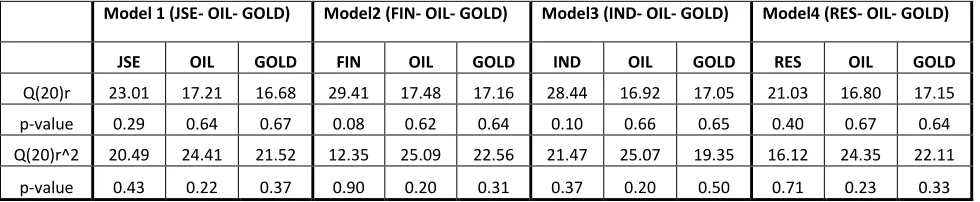
Table 5 below represents the diagnostic tests for the estimated models. The Q-statistics test in table
5 confirms that the null hypothesis of no autocorrelation (also known as serial correlation) is not
rejected for the estimated VAR-ADCC-GARCH (1, 1) model. Therefore, the estimated model is
specified correctly for modelling the dynamic link between stock, oil and gold returns. Thus, we
MODEL 1 (JSE- OIL- GOLD) MODEL 2 (FIN- OIL- GOLD) MODEL 3 (IND- OIL- GOLD) MODEL 4 (RES- OIL- GOLD)
Coefficient SE Coefficient SE Coefficient SE Coefficient SE
Mean Eq
𝑪𝟏 0.0203 0.0148 0.0321** 0.0154 0.0576*** 0.0130 -0.0228 0.0289
𝝎𝟏𝟏 -0.0236 0.0183 -0.0025 0.0201 -0.0114 0.0192 -0.0206 0.0188
𝝎𝟏𝟐 0.0537*** 0.0099 0.0073 0.0099 0.0278*** 0.0087 0.1126*** 0.0176
𝝎𝟏𝟑 0.0015 0.0141 -0.0254* 0.0152 -0.0108 0.0143 0.0187 0.0260
𝑪𝟐 -0.0203 0.0248 -0.0143 0.0254 -0.0137 0.0255 -0.0143 0.0340
𝝎𝟐𝟏 0.0261 0.0267 0.0311 0.0279 0.0251 0.0306 0.0153 0.0191
𝝎𝟐𝟐 -0.0637*** 0.0199 -0.0633*** 0.0187 -0.0620*** 0.0171 -0.0572** 0.0227
𝝎𝟐𝟑 0.0062 0.0226 0.0041 0.0251 0.0035 0.0235 0.0079 0.0274
𝑪𝟑 0.0110 0.0218 0.0160 0.0201 0.0174 0.0206 0.0127 0.0240
𝝎𝟑𝟏 0.0220 0.0189 0.0144 0.0182 0.0126 0.0221 0.0192 0.0122
𝝎𝟑𝟐 0.0399*** 0.0107 0.0418*** 0.0115 0.0410*** 0.0107 0.0386*** 0.0119
𝝎𝟑𝟑 -0.0187 0.0211 -0.0140 0.0252 -0.0168 0.0228 -0.0250 0.0249
Variance Eq
𝝋𝟏 0.0145*** 0.0040 0.0231*** 0.0049 0.0261*** 0.0037 0.0270*** 0.0089
𝝋𝟐 0.0103 0.0070 0.0104* 0.0061 0.0088 0.0075 0.0126 0.0115
𝝋𝟑 0.0164 0.0148 0.0163 0.0139 0.0136 0.0144 0.0175 0.0117
𝜶𝟏𝟏 0.0024 0.0106 0.0266*** 0.0088 0.0012 0.0050 0.0215 0.0144
𝜶𝟏𝟐 -0.189*** 0.0060 -0.0098 0.0077 -0.015** 0.0005 0.1905** 0.0101
𝜶𝟏𝟑 -0.0079 0.0078 -0.0330 0.0894 -0.0169* 0.0095 0.0118*** 0.0011
𝜶𝟐𝟏 -0.0134 0.0122 -0.0023 0.0167 -0.0125 0.0211 -0.0154 0.0285
𝜶𝟐𝟐 0.0248*** 0.0048 0.0243*** 0.0048 0.0244*** 0.0058 0.0304** 0.0136
𝜶𝟐𝟑 -0.0190* 0.0097 -0.0217* 0.0131 -0.0211 0.0137 -0.0208 0.0199
𝜶𝟑𝟏 -0.0244 0.0166 -0.0030 0.0126 -0.0350 0.1534 -0.0132 0.0102
𝜶𝟑𝟐 -0.0038 0.0089 -0.0053 0.0096 -0.0023 0.0087 -0.0069 0.0086
𝜶𝟑𝟑 0.0516*** 0.0131 0.0503*** 0.0110 0.0472*** 0.0129 0.0539*** 0.0139
𝜷𝟏𝟏 0.9061*** 0.0139 0.8999*** 0.0120 0.9006*** 0.0121 0.9303*** 0.0219
𝜷𝟏𝟐 0.0360*** 0.0115 0.0111 0.0142 0.209** 0.0096 0.9054*** 0.0147
𝜷𝟏𝟑 0.0198 0.0205 0.0228 0.0282 -0.0401 0.2063 0.0689** 0.0337
𝜷𝟐𝟏 0.0141 0.0138 -0.0044 0.0315 0.0105 0.0353 0.0455 0.0816
𝜷𝟐𝟐 0.9439*** 0.0052 0.9454*** 0.0041 0.9453*** 0.0080 0.9303*** 0.0282
𝜷𝟐𝟑 0.0594*** 0.0197 0.0637** 0.0301 0.0650** 0.0263 0.0467 0.0585
𝜷𝟑𝟏 0.0268 0.0315 0.0333 0.0239 0.0217 0.0337 0.0276* 0.0161
𝜷𝟑𝟐 0.0271 0.0248 0.0239 0.0303 0.0205 0.0270 0.0272 0.0268
𝜷𝟑𝟑 0.9288*** 0.0359 0.9333*** 0.0330 0.9391*** 0.0333 0.9209*** 0.0341
𝜸𝟏 0.1359*** 0.0153 0.1181*** 0.0098 0.1347*** 0.0099 0.0799*** 0.0124
𝜸𝟐 0.0464*** 0.0092 0.0459*** 0.0097 0.0450*** 0.0084 0.0472*** 0.0163
𝜸𝟑 0.0006 0.0300 -0.0006 0.0261 -0.0008 0.0246 0.0021 0.0264
𝒇𝟏 0.0172*** 0.0035 0.0191*** 0.0046 0.0172*** 0.0016 0.0220* 0.0125
𝒇𝟐 0.9747*** 0.0063 0.9664*** 0.0095 0.9706*** 0.0048 0.9627*** 0.0391
can proceed to the construction of time-varying conditional correlations, portfolio weights and
[image:24.612.72.562.140.241.2]hedge ratios from the estimated model.
Table 5: Diagnostics Tests for Standardised Residuals
Model 1 (JSE- OIL- GOLD) Model2 (FIN- OIL- GOLD) Model3 (IND- OIL- GOLD) Model4 (RES- OIL- GOLD)
JSE OIL GOLD FIN OIL GOLD IND OIL GOLD RES OIL GOLD
Q(20)r 23.01 17.21 16.68 29.41 17.48 17.16 28.44 16.92 17.05 21.03 16.80 17.15
p-value 0.29 0.64 0.67 0.08 0.62 0.64 0.10 0.66 0.65 0.40 0.67 0.64
Q(20)r^2 20.49 24.41 21.52 12.35 25.09 22.56 21.47 25.07 19.35 16.12 24.35 22.11
p-value 0.43 0.22 0.37 0.90 0.20 0.31 0.37 0.20 0.50 0.71 0.23 0.33
Note: Q(20)r and Q(20)r^2 represent the Ljunge-Box test statistics of up to 20 lags for standardised and squared standardised residuals.
4.2.2 Time-varying Conditional Correlations
In this section, we analyse the time-varying correlations for specific pairs of oil and
stock-gold portfolios13 obtained from the VAR-ADCC-GARCH model estimated above. Understanding
the co-movement between a commodity and the stock markets returns is crucial for portfolio and
risk management. Indeed, the traditional asset pricing theory states that portfolio diversification
gains are associated with the correlation of assets included in the diversified portfolio. Thus,
combining negatively or low positively correlated assets might help reduce the average volatility
of a portfolio, as the shifts in one asset can be expected, at the very least, to be reduced by shifts
in the other asset.
We will examine how the correlations between stock market returns and commodity futures evolve
during normal times as well as during periods of financial turmoil. The reason why we evaluate
the correlation between the stock markets and commodities during periods of financial turmoil is
because during these periods stock markets tend to be highly volatile (see figure 1 above).
Therefore, in order to diversify the high risk associated with these periods of crises, which is when
portfolio diversification benefits are needed the most, we need to understand how the two assets
co-move. The sample used in this study incorporates two crises periods, namely, the global
financial crises and the Eurozone sovereign debt crisis.
13 Note: this paper mainly focuses on stock-gold and stock-oil portfolios, unless stated otherwise. We do so because
Before we analyse our results on dynamic correlations, it is important to distinguish between a
portfolio diversifier, a hedge and a safe haven. A definition we can consider to be useful in guiding
the reader through the rest of this study is that provided by Baur and Lucey (2010), and is as
follows;
A diversifier is defined as an asset that is positively (but not perfectly
correlated) with another asset or portfolio on average. A hedge is defined
as an asset that is uncorrelated or negatively correlated with another asset
or portfolio on average. And a safe haven is defined as an asset that is
uncorrelated or negatively correlated with another asset or portfolio in
times of market stress or turmoil.
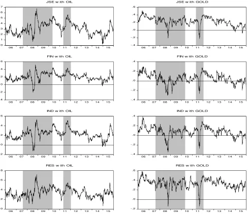
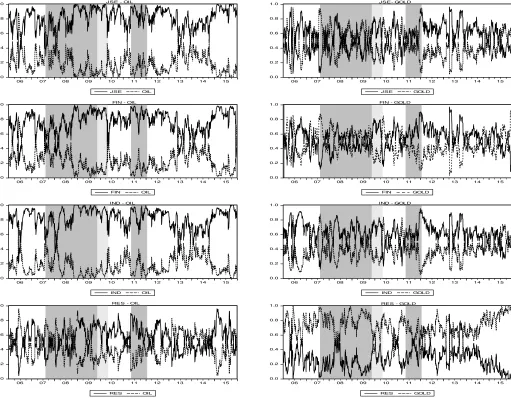
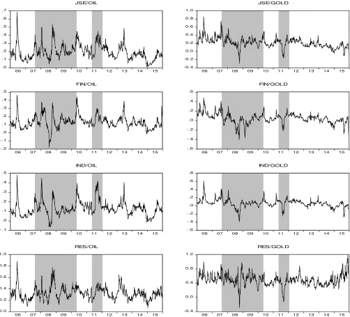
Figure 2 below illustrates the time-varying correlations for the specific stock-oil and stock-gold
pairs under study. The time-varying correlations seem to be highly volatile over time, indicating
that relying solely on static correlations to estimate optimal weights and hedge ratios might be
misleading. The correlation for most stock-oil and stock-gold pairs under study seems to be
relatively close to their respective unconditional correlations (shown in table 2). In addition, it is
interesting to note that the correlation for all pairs under study drastically changes during periods
of crisis. This finding is similar to that of most empirical studies (Arouri et al., 2011; Kang et al.,
2016), showing that the correlation between stock markets and commodities significantly changes
during periods of extreme uncertainty.
Regarding the dynamic correlation between oil and stock markets, the pattern seems similar for
the JSE-OIL, FIN-OIL and IND-OIL pairs. For the FIN-OIL and IND-OIL pairs, we notice that
the correlation fluctuates between positive and minuscule negative values. During the global
financial crisis, which commenced at the end of 2007 or the beginning of 2008, there were negative
values of -0.2 for FIN-OIL and -0.1 for IND-OIL. However, during this period, the negative
correlation of FIN-OIL and IND-OIL pairs was only temporary (lasting approximately one month,
according to our results), as the correlation for both pairs rose dramatically to positive territory
(reaching +0.5) when the crisis became more severe. As noted above, the correlation between the
aggregate JSE and OIL follows a similar pattern to that of the FIN-OIL and IND-OIL pairs.
However, unlike in case of the FIN-OIL and IND-OIL pairs, the correlation between the JSE and
FIN-OIL and IND-FIN-OIL pairs, the correlation between JSE-FIN-OIL also drops at the end of 2007 and the
beginning of the 2008 when the global crisis really emerged, showing a low positive correlation
of +0.07, which then rose to +0.7 when the crisis was in full force.
These findings on the co-movement between the stock markets (excluding resources sector) and
oil should be expected in the case of South Africa. At the beginning of 2008, the global financial
crisis resulted in a negative economic growth in most economies around the world, which led to a
decline in demand for oil and a large drop in oil prices. However, at the beginning of 2008, some
emerging markets (particularly South Africa) were not yet affected by the global financial crisis
(as developed markets were). Therefore, the high volatility in developed stock markets, which
signalled a high degree of market risk, may have led to foreign market participants seeking more
stable equity markets and higher returns to relocate from developed markets to developing
markets. This movement resulted in South African stock prices increasing and moving in the
opposite direction to oil, hence the negative correlation between the two assets (oil and stock
market prices) at the beginning of 2008. However, as soon as the crisis hit South Africa (which
was in the third quarter of 2008), domestic stock markets also dropped significantly, resulting in
the two variables (oil and stock market prices) moving in the same direction, hence the increase in
correlation when the crisis escalated.
Similarly, the correlation between stock-oil pairs during the Eurozone sovereign debt crisis in 2011
also rose to significantly higher positive values. This high positive correlation between oil and the
stock market prices is not surprising, because they are usually linked to economic conditions and
variables (Souček, 2013). In contrast, the RES-OIL pair seems to have exhibited a different
correlation pattern compared to other stock market sectors with regard to oil. For RES-OIL, we
notice that the correlation between RES and OIL fluctuation around positive values for the sample
period under study. Moreover, the correlation between RES and OIL increases significantly to
high positive values during both periods of crisis. The positive correlation between RES and OIL
is understandable, as the resources sector index includes oil companies whose profits depend on
the price of crude oil.
Regarding the correlation between gold and the stock markets, our results reveal a similar pattern
for all gold-stock pairs (except RES-GOLD). In contrast to the stock-oil pairs’ correlation, the
during both periods of crisis highlighted in this paper. It is also important to note that the decline
in the stock-gold pairs’ correlation began to decline before the crisis hit South Africa, and
continued during the financial crisis, because gold prices tend to react positively to negative
financial or economic news. Therefore, this could be a potential indication that gold may be a safer
asset, as a change in gold prices tends to have an inverse relationship with stock market returns
during periods of crisis in most cases. Moreover, gold might also a good hedge against stock
market exposure because of its low correlation with the stock markets over time. Our results are
somewhat similar to those of previous studies by Baur and Lucey (2010) and Ciner et al. (2013),
which also suggest that gold has the qualities of a good hedge and a safe haven tool.
However, the RES-GOLD pair correlation seems to exhibit a different trend when compared with
other stock market sectors’ relationship to gold. For RES-GOLD, we notice that the correlation
between the resources sector and gold is exceptionally high over time, because the resources sector
includes mining shares, which usually co-move with gold prices. In addition, during both crisis
periods under study, the correlation declined to a negative territory for a short period of time, then
reverted to high positive territory. The reason for the short-term drop in correlation may be owing
to the fact that resources’ shares were still classified as ‘risky assets’ and, during crisis periods,
investors avoid investing in risky assets. However, since the resource companies benefit from high
gold prices (especially from South Africa as a gold-producing country) during a crisis period, the
correlation reverted to positive territory.
Table 6 below presents a summary of statistics for dynamic conditional correlations. In this table,
we notice that the correlations for all oil-stock and gold-stock pairs vary between a minimum of
−0.35 (IND/GOLD) and a maximum of +0.72 (RES/OIL). Therefore, during periods of negative
correlation (as shown in figure 2 for all pairs under study), there is an opportunity for meaningful
portfolio diversification.
Our dynamic correlation results provide some information regarding portfolio diversification.
Firstly, the correlation between crude oil futures and the South African stock markets (excluding
the resources sector) mostly fluctuates below +0.5 during normal times. This fluctuation is a sign
that oil could be a useful hedge instrument against the stock markets’ exposure during normal
times. However, during periods of financial distress, the correlation between crude oil futures and
indicate that oil might not be a good hedge or a safe haven against stock markets’ exposure, proving that there is limited scope for portfolio diversification for stock-oil portfolios during periods of
financial or economic crisis when diversification benefits are needed the most.
Secondly, the correlation between gold futures and the South African stock markets (excluding the
resources sector) mostly fluctuates below +0.4 during normal times. This fluctuation is a sign that
gold could be a useful hedge instrument against stock markets’ exposure during normal times.
Moreover, during periods of financial turmoil, the correlation between gold futures and the South
African stock markets increases significantly, reaching negative values. This shift is consistent
with the evidence provided by Baur and Lucey (2010) that indicates that gold might be a good
hedge and safe haven against stock markets’ exposure.
Thirdly, with regards to the correlation between gold or crude oil futures with the resources sector,
we notice that the correlation is mostly positive and high. As noted above, this correlation makes
economic sense, as the resources sector includes mining, and oil companies co-move with
commodity prices (gold and oil in particular). Therefore, our results suggest that commodities (oil
and gold) may provide a neither a good hedge nor safe haven for resources stock price risk. Further
research on this matter is conducted below.
In conclusion, our results are consistent with findings of Kang et al. (2016), who also indicated
that oil could be a hedge against emerging stock market exposure, but there is little scope for
portfolio diversification for oil and the stocks portfolio during periods of financial distress. This
study by Kang et al. also shows evidence that gold can play the role of a safe haven and hedge
[image:28.612.78.499.561.705.2]against stock markets’ exposure during periods of financial distress.
Table 6: Summary Statistics of Time-varying Conditional Correlations
PORTFOLIO MEAN STANDARD DEVIATION MINIMUM MAXIMUM JSE/OIL 0.3103 0.1092 0.0212 0.6746
JSE/GOLD 0.2262 0.1123 -0.2291 0.5103
FIN/OIL 0.2047 0.0977 -0.1997 0.5196
FIN/GOLD 0.0501 0.1025 -0.3070 0.2984
IND/OIL 0.2254 0.1050 -0.1275 0.5345
IND/GOLD 0.0745 0.1026 -0.3506 0.3930
RES/OIL 0.3405 0.0929 0.0639 0.7216