A Mathematical Approach Based on the Homotopy Analysis Method: Application to Solve the Nonlinear Harry Dym (HD) Equation

http://www.scirp.org/journal/am ISSN Online: 2152-7393 ISSN Print: 2152-7385

DOI: 10.4236/am.2017.811113 Nov. 13, 2017 1546 Applied Mathematics

A Mathematical Approach Based on the

Homotopy Analysis Method: Application to

Solve the Nonlinear Harry-Dym (HD) Equation

Emran Khoshrouye Ghiasi, Reza Saleh

*

Department of Mechanical Engineering, College of Engineering, Mashhad Branch, Islamic Azad University, Mashhad, Iran

Abstract

In this paper, the homotopy analysis method (HAM) has been employed to obtain the approximate analytical solution of the nonlinear Harry-Dym (HD) equation, which is one of the most important soliton equations. Utilizing the HAM, thereby employing the initial approximation, variations of the 7th-or- der approximation of the Harry-Dym equation is obtained. It is found that ef-fect of the nonzero auxiliary parameter on convergence rate of the series solu-tion is undeniable. It is also shown that, to some extent, order of the fracsolu-tional derivative plays a fundamental role in the prediction of convergence. The final results reported by the HAM have been compared with the exact solution as well as those obtained through the other methods.

Keywords

Harry-Dym (HD) Equation, Soliton, Homotopy Analysis Method (HAM), Auxiliary Parameter, Convergence Analysis, Relative Error

1. Introduction

The nonlinear Harry-Dym equation is [1],

3 _,

t xxx

u =u u (1)

with the initial approximation,

( )

2 3

3

, 0 ,

2 b u x =_a− x_

  (2) where a and b are constants.

Equation (1) is one of the most important soliton equations i.e., a soliton is

How to cite this paper: Khoshrouye Ghia-si, E. and Saleh, R. (2017) A Mathematical Approach Based on the Homotopy Analy-sis Method: Application to Solve the Non-linear Harry-Dym (HD) Equation. Applied Mathematics, 8, 1546-1562.

https://doi.org/10.4236/am.2017.811113

Received: October 3, 2017 Accepted: November 10, 2017 Published: November 13, 2017

Copyright © 2017 by authors and Scientific Research Publishing Inc. This work is licensed under the Creative Commons Attribution International License (CC BY 4.0).

http://creativecommons.org/licenses/by/4.0/

DOI: 10.4236/am.2017.811113 1547 Applied Mathematics deemed as solitary, travelling wave pulse solution of nonlinear partial differential equations (NPDEs) [2] e.g., the Korteweg-de Vries (KdV) equation (see Refs. [3] [4]). Moreover, according to Drazin and Johnson [5], a soliton can interact strongly with other solitons and retain its identity. Among the efforts and achievements due to the behavior of the Harry-Dym equation, Popowicz [6] ge-neralized this equation by the Lax and Hamiltonian formulations. He also found that generalization of the Harry-Dym Lax operator is only limited to two opera-tors. As reported by Marciniak and Błaszak [7], if a classical Stäckel system is applied to construct the coupled Harry-Dym (cHD) hierarchy, both nonlocal and purely differential parts of hierarchies are obtained. Using the Riemann- Liouville derivative, Huang and Zhdanov [8] recently investigated the time frac-tional nonlinear Harry-Dym equation with the Lie symmetry and obtained some invariant solutions explicitly. Brunelli and da Costa [9] studied a large class of nonlocal equations and charges for the Harry-Dym hierarchy. Tian and Liu [10]

presented a new non-trivial supersymmetric Harry-Dym equation using the su-persymmetric reciprocal transformation. Ma [11] constructed an extended Har-ry-Dym hierarchy using a sequence of Lax equations with the new time variables. However, this extended Harry-Dym equation which is based on the adjoint ei-genfunctions, have not been taken into account by Wu et al.[12]. In other words, Wu et al.[12] proposed a 2+1 dimensional Harry-Dym hierarchy and found that this extended scheme is Lax integrable. It should be noted that more details on the Harry-Dym equation are available in Refs. [13][14].

This paper is organized as follows. Section 2 gives an overview of the HAM. In Section 3, the HAM is applied to solve the nonlinear Harry-Dym equation with the initial approximation given in Equation (2). Section 4 is devoted to the re-sults and discussion. Concluding remarks are given in Section 5.

2. Homotopy Analysis Method (HAM)

The essence of the HAM [15]-[20] is based on the approximation of PDEs along with a convenient way to guarantee convergence of the series solution. This issue can be outlined by the following example.

Consider the following nonlinear differential equation,

( )

, 0,

A u x t_ _= (3)

in which A is a nonlinear operator, x and t are independent variables and

( )

,

u x t is an unknown function. On account of a continuous mapping from

( )

,

(

, ;

)

u x t →ϕ x t p , the homotopy embedding parameter p varies from 0 to 1; it

means that ϕ

(

x t p, ;

)

varies from the initial approximation u₀

( )

x t, to the

exact solution u x t

( )

, . This mapping is constructed by the zeroth-order

defor-mation equation which is defined as,

(

1−p L

)

ϕ

(

x t p, ;

)

−u0

( )

x t, =phH x t A

( )

, ϕ

(

x t p, ;

)

, (4)

in which L is a linear operator, h≠0 is an auxiliary parameter and H x t

( )

, is

DOI: 10.4236/am.2017.811113 1548 Applied Mathematics

A) with respect to p gives,

(

)

(

)

1

(

)

0

, ; 1

, ; , ; 0 ,

! m m m m p x t p

x t p x t p

m p

ϕ

ϕ

ϕ

∞

= =  ∂  = + _ _ ∂  

∑

(5)

or,

(

, ;

)

0

( )

, 1

( )

, . m m

m

x t p u x t u x t p

ϕ ∞

=

= +

∑

(6)

If L, h, H x t

( )

, and u0

( )

x t, are properly chosen, the power series (6)

converges at p=1, then one has,

(

x t, ;1

)

u0

( )

x t, m1um

( )

x t, ,

ϕ ∞

=

= +

∑

₍₇₎

which must be one of the solutions of Equation (3), as proved by Liao [15]. Now, it is of particular interest to show that Equation (7) provides a relationship be-tween the initial approximation and the exact solution so that:

1) Solution of Equation (4) is valid for p∈

[ ]

0,1 .

2) The deformation derivative

(

)

0

, ; m

m p x t p

p

ϕ

= ∂     _∂ 

  exists for all values of m. Differentiating the zeroth-order deformation Equation (4) m times with re-spect to p, then setting p=0 and dividing them by m!, gives the so-called

mth-order deformation equation as,

( )

, 1

( )

,

( )

, 1

( )

, ,

m m m m m

L u_ x t −χ u ₋ x t _=hH x t R _u ₋ x t _ (8)

in which, 0, 1, 1, 1, m m m

χ _{= } ≤

>

 (9) and,

( ) ( )

1

(

)

1 1 0 , ; 1 , . 1 ! m

m m m

p

A x t p

R u x t

m p ϕ − − − = ∂ _ _ =       _{−  ∂ }

  (10)

It should be noted that u_m

( )

x t, for m≥1 is governed by the linear

Equa-tion (8) with the linear boundary condiEqua-tions that come from the original prob-lem, which can be easily solved using some software programs such as MAPLE or MATHEMATICA.

DOI: 10.4236/am.2017.811113 1549 Applied Mathematics integral equations of the second kind. They also used the auxiliary parameter to show influence of this parameter on the convergence rate. In a book, current advances of the HAM to solve strongly nonlinear problems were edited by Liao

[24]. Ren et al.[25] introduced an approximate analytical solution to the Gross- Pitaevskii equation while a nonlinear Schrödinger equation was utilized to si-mulate Bose-Einstein condensates trapped in a harmonic potential. Martin [26]

proposed an analytical algorithm to solve an integral-differential equation of the transport theory for stationary case using HAM. The solution of nonlinear boundary value problems (NBVPs) based on the Chebyshev operational matric-es was invmatric-estigated by Shaban et al.[27]. They applied the Tau method to con-vert a set of algebraic equations so that the solution can be obtained iteratively. Motsa et al. [28] utilized the spectral-homotopy analysis method (SHAM) to solve the Darcy-Brinkman-Forchheimer equation and found the admissible range of auxiliary parameter for this problem. Hesameddini and Latifizadeh [29]

obtained solutions for the first and second types of the Painlevé equations with 8, 10 and 12 iterations. Wang [30] developed an approximate analytical solution of relativistic Toda lattice system and concluded that using HAM may be very ef-fective for solving differential difference equations (DDEs). In other words, some papers are devoted to compare the HAM with the other analytical methods e.g., optimal homotopy asymptotic method (OHAM), differential transforma-tion method (DTM), homotopy perturbatransforma-tion method (HPM), general series ex-pansion method, harmonic balance method (HBM) which can be found in Refs.

[31][32][33][34][35].

3. HAM Formulation for the Nonlinear Harry-Dym Equation

As mentioned above, the Equation (1) can be solved through the HAM. To this end, the linear operator takes the form of,

(

, ;

)

(

x t p, ;

)

,

L x t p

t ϕ

ϕ =∂

 

  _∂ (11)

with the property,

[ ]

0,

L d = (12)

in which d is an integral constant. Now the nonlinear operator can be expressed in terms of Equation (1) as,

(

)

(

)

(

)

3 3

(

)

3

, ; , ;

, ; x t p , ; x t p .

A x t p x t p

t x

ϕ ϕ

ϕ =∂ − ϕ ×∂

   

  _∂   _∂ (13)

Using the above definition, with the assumption H x t

( )

, =1, the zeroth-order

deformation can be given as,

(

1−p L

)

ϕ

(

x t p, ;

)

−u0

( )

x t, =phAϕ

(

x t p, ;

)

. (14)

For p=0 and p=1, it is respectively written as,

(

x t, ; 0

)

u0

( )

x t, u x

( )

, 0 ,

DOI: 10.4236/am.2017.811113 1550 Applied Mathematics

(

x t, ;1

)

u x t

( )

, .

ϕ = (15b) Herein, the 𝑚𝑚th-order deformation equation is given by,

( )

, 1

( )

, 1

( )

, ,

m m m m m

L u_ x t −χ u ₋ x t _=hR _u ₋ x t _ (16)

in which,

( )

1

( )

1

( )

3 3 1

( )

1 0 3

, ,

, m m , m .

m m n n

u x t u x t

R u x t u x t

t x − − − − = ∂ ∂ = − ×    

  _∂

∑

  _∂ (17)

It should be noted that the discretized form of above equation is illustrated in

Appendix B. So, solution of the 𝑚𝑚th-order deformation equation for m≥1

can be expressed by,

( )

( )

1

{

( )

}

1 1

, , , .

m m m m m

u x t =χ u ₋ x t +hL− R _u ₋ x t _ (18) Now, according to Equation (18), the values of um

( )

x t, for m=1, 2, can

be obtained as,

( )

1 3 3 2 1 3 , , 2 b

u x t htb a x

−

 

= _ − _

  (19a)

( )

1 3 1 3

3 2 2 3 2

2

4 3 13 3

2 2 3 5 5 15 2

3 3

,

2 2

7 3 7 3

2 2

2 3 2 3 ,

b b

u x t htb a x h tb a x

b b

h t b a x h t b a x

− − − −     = _ − _ + _ − _         − _ − _ − _ − _     (19b)

( )

1 3 1 3

3 2 2 3 2

3

4 3 13 3

2 2 3 5 5 15 2

1 3 1 3

2 3 2 3 3 2

4 3

3 2 3 6 5 15 2

3 3

,

2 2

7 3 7 3

2 2

2 3 2 3

3 3

2 2

7 3 35 3

2

3 2 3

b b

u x t htb a x h tb a x

b b

h t b a x h t b a x

b b

h tb a x h tb a x

b b

h t b a x h t b a

− − − − − − −     = _ − _ + _ − _         − _ − _ − _ − _         + _ − _ − _ − _       − _ − _ − −   13 3 2 x −        

2 10 3

2 2 3

10 3 13 3

3 2 3 3 3 9 2

3

22 3 1 3

6 6 9 3 2

10 3 2 2 3

3 7 3

2 2 2

7 3 245 3

2 2 2 3 2

1729 3 3

2 2

3

7 3

2 2

b b

a x h t b a x

b b

h t b a x h t b a x

b b

h t b a x htb a x

b

h t b a x

− − − − − −       −_ − _ × _ − _    _       + _ − _ − _ − _               − _ − _ − _ − _      _{ }   _  _{ } × _ − _    10 3 3 2 3

7 3

2 2

b

h t b a x

−

 

 + _ − _

 _{ }

DOI: 10.4236/am.2017.811113 1551 Applied Mathematics

13 3 22 3

3 3 9 2 6 6 9

3

13 3 10 3

5 5 15 2 2 2 3

10 3 13 3

3 2 3 3 3 9 2

245 3 1729 3

2 2

2 3 3

7 3 7 3

2 2 2

2 3

7 3 245 3

2 2 2 3 2

1729 3

b b

h t b a x h t b a x

b b

h t b a x h t b a x

b b

h t b a x h t b a x

h

− −

− −

− −



   



− _ − _ − _ − _



    _

 _{ }   _{ }

  

− _ − _ × _ − _

 _{ }   _{ }

  

   

+ _ − _ − _ − _

   

−

22 3

6 6 9 3

. 2

b

t b a x

− _

 

 −

 

  _

  _

To continue this procedure for m>3, u_m

( )

x t, can be achieved and the

se-ries solution is completely computed.

4. Results and Discussion

4.1. Comparison and Validation

To validate the present iterative approach, results are compared with the exact solution of the Harry-Dym equation provided by Mokhtari [36] which can be expressed as,

( )

(

)

2 3

3

, 1 ,

2 b

u x t = − x+ct 

 

  (20)

where c is a constant. Mokhtari [36] also showed that the variational iteration method (VIM) is not able to obtain implicit solution of the Harry-Dym equation. However, one should point out that Hereman et al.[37] proposed implicit solu-tion of this equasolu-tion via a direct method and also performed transformasolu-tions between the Harry-Dym and KdV equations explicitly. In particular, according to the fractional Harry-Dym equation,

3

, t xxx

uα =u u (21)

[image:6.595.274.528.74.233.2]

where 0≤ ≤α 1 is a parameter describing order of the fractional derivative,

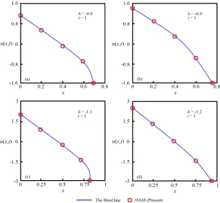
Figure 1 depicts variations of u x t

( )

, versus x for the Harry-Dym equation

calculated by different methods. As shown in this figure, variation of u x t

( )

,

predicted by the HAM is in good agreement with those provided by Mokhtari

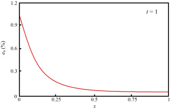
[36]. However, there is a relative error between the results which can be calcu-lated by,

( )

%

( ) ( )

,

( )

, 100, ,

u

u x t u x t e

u x t

−

= × (22)

where u x t

( )

, and u x t

( )

, are the exact and approximate solutions of

[image:7.595.235.512.74.247.2]

DOI: 10.4236/am.2017.811113 1552 Applied Mathematics Figure 1. Variation of u x t

( )

, versus x for 7th-order approximation of the nonlinear Harry-Dym equation with the HAM and compared with those reported in Refs. [36] [38] [39] [40] [41].

Figure 2. Depiction of discrepancy (i.e., error) between the present iterative method and exact solution due to Equation (22).

approach, i.e.,

( ) ( )

( )

2

1

, ,

1

, n

i

u x t u x t

n = u x t

 − 

 

 

 

∑

[42], is also 0.509%. Apart from the

exact solution, other observations may be made from Figure 1; e.g., it is assumed that for h= −1, the series solution will be converged at the results presented in

[image:7.595.235.514.310.489.2]

sug-DOI: 10.4236/am.2017.811113 1553 Applied Mathematics gested largely due to its less time-consuming and also is able to obtain valid val-ues of the auxiliary parameter. However, it should be noted here that although we utilize h= −1 in our solution, the convergence can be observed when the objective is to replace Equation (21) by Equation (1) for α=1.

Another comparison is also performed here to illustrate the accuracy of present iterative approach when the effect of nonlinearity has been taken into account. In connection with this matter, Rawashdeh [40] utilized the fractional reduced differential transformation method (FRDTM) to solve the nonlinear Harry-Dym equation while the maximum error between the HAM and FRDTM for u x t

( )

, is 11.723%. In addition, He found that u x t

( )

, predicted by the

FRDTM is on average 1.18 less than that predicted by exact solution and is greatly affected by the number of iterations performed. Based on this compari-son, it is seen that Equation (21) without α=1 would also fit into HAM,

namely, Caputo sense [45], which is not correspondent to define the fractional order initial conditions. Herein, the Caputo’s formula is defined as [46],

(

)

( )

(

1

) (

)

1 ( )

( )

d , 1 , , 0.

Γ

x m m

a _a

D u x x u m m m N x m

α

α _{τ τ τ α}

α

− −

+ = ₋

∫

− − < ≤ ∈ > (23)

It should be noted that Kumar and Singh [41] applied the Laplace transform on the both sides of Equation (21) and solved the governing equation through a homotopy perturbation transform method (HPTM), but their solution could not capture u x t

( )

, especially for the cases with large values of auxiliary parameter.

There exists a discrepancy between the exact solution and those obtained through HPTM because of decomposing the nonlinear term in He’s polynomial (i.e., Equation (17)). To clarify, the He’s polynomial has been also used in some previous studies [47][48]. It is to be noted that Guo and Mei [47] studied time- fractional Boussinesq-type equation by the VIM and Khan and Wu [48] investi-gated the advection problems through HPTM.

4.2. Universal Graphs for Convergence Region of the Presented

Iterative Approach

The fact that Equation (18) is not convergent for all values of the auxiliary para-meter, lifts some particular restrictions on choosing a proper value of h∈

(

h h1, 2

)

(e.g., by trial and error [49]). Above all, making a good selection of h is impor-tant not only with the convergence, but also with the basis functions [16][50]. It should be noted that other perturbation methods require the need for small pa-rameters, which may commonly diverge series solutions with slight changes (see Ref. [17]). Indeed, at large values of the auxiliary parameter, convergence may lead to only few terms of series solution. It is shown that based on the zeroth- order deformation Equation (4), one may expect the flexibility and freedom to select L, despite the fact that the order of linear operator will be different from the original nonlinear problem (see Ref. [50]). As said in Ref. [49]

DOI: 10.4236/am.2017.811113 1554 Applied Mathematics fixed choice of the initial approximation, auxiliary linear operator and auxiliary function.”

—R.A. Van Gorder and K. Vajravelu [49]

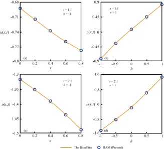
Due to Figure 1 that u x t

( )

, varies almost linearly versus x, Figure 3 shows

the variation of u x t

( )

, for some different auxiliary parameters. It is seen that

1

h< − indicates the ascending behavior while h> −1 suggests the descending behavior of the present iterative approach. Although the slopes of these lines are slightly different from each other, the lines become parallel by increasing or de-creasing the auxiliary parameter in the neighbourhood of h= −1. It should be noted that this fact can result in almost linear variation of u x t

( )

, . In theory, at

the mth-order of approximation, the square residual error can be defined as

[51],

( )

{

}

2

0

0 d .

m

m A i ui τ τ

∞

=

 

∆ =

∫

_

∑

_ (24) [image:9.595.214.533.401.694.2]

It should be noted that as ∆m decreases to zero more rapidly, the conver-gence rate for corresponding series solution would become faster [51]. In this regard, Yabushita et al.[52] introduced an analytical approximation to projectile motion with the quadratic resistance law by the HAM. They derived governing equations using a power series which was accurate enough for large angle of projection. Therefore, with a minimum value of ∆m, the optimal values of un-known auxiliary parameters were obtained.

DOI: 10.4236/am.2017.811113 1555 Applied Mathematics It should be noted that by increasing t, u x t

( )

, will be decreased slightly, as it

is shown in Figure 4(a) and Figure 4(c). It is mainly due to the fact that this parameter plays an important role in higher-order governing equations (e.g., Equation (19c)) (see Refs. [22] [33] [53] [54]). It is to be noted that a similar conclusion for increasing t can also be drawn through a similar procedure. Odi-bat [55] reached a pragmatic approach for the convergence of HAM, and to date, no counterexample exits in the open literature for this conclusion, neither for NPDEs nor for PDEs. Hence, in such graphs we increase t from 1 to its a neigh-borhood which can exhibit this deviation for a better presentation. However, it is to be noted that this parameter is small in most of the analytical approximations (e.g., 0≤ ≤t 2) [18][19][49].

According to the higher-order equations (e.g., Equation (19c)), if t will be in-creased, the maximum value of u x t

( )

, will be increased for − ≤ ≤1 h 1 (see

Figure 4(b) and Figure 4(d)). It is noted that u x t

( )

, almost drops to zero

when the auxiliary parameter reaches to zero as well. It is seen that neglecting the effect of t may lead to underestimation of u x t

( )

, versus h. However, if this

parameter exceeds its t1, which can be named as a minimum value of t,

( )

,

u x t will be fully negative.

[image:10.595.209.537.400.697.2]

It is noteworthy to mention that although many techniques (e.g., HPM, ADM, FRDTM, HPTM) can be useful for predicting analytical approximations of the nonlinear Harry-Dym Equation (1), the more accurate results can be obtained

DOI: 10.4236/am.2017.811113 1556 Applied Mathematics through the HAM. On the other hand, since the HAM is employed to approx-imate NPDEs analytically, it is important to note that it enables us to construct a mapping of initial approximation to the exact solution of nonlinear governing equation.

5. Concluding Remarks

In this paper, the nonlinear Harry-Dym equation, which describes a couple of nonlinearity and dispersion, has been solved iteratively. It has been shown that Equation (1), which can be transformed to the KdV equation, is an integrable NPDE. Furthermore, it has been shown that the HAM is an efficient method which provides a convenient way to guarantee convergence of the series solu-tions. The main inferences that can be drawn from this work are summarized as follows:

• _{The HAM will enable us to make an informed choice for auxiliary linear} op-erator and initial approximation which can be employed to obtain the series solution.

• _{Equation (18) indicates one important role of the auxiliary parameter which} was introduced to construct the zeroth-order deformation Equation (4). • _{Convergence of the power series (6) largely depends on the range of auxiliary}

parameter.

• _{In case of} h= −1, the HPM is a special case of HAM, as proved by Liao [56].

• _{By using} H x t

( )

, =1, influence of the auxiliary function, with the exception

of some particular recursive problems (see Ref. [49]) will be neglected. • _{Presence of}

α

affects u x t

( )

, considerably when the fractional Harry-

Dym equation is utilized.

References

[1] Kruskal, M.D. and Moster, J. (1975) Dynamical Systems: Theory and Applications, Lecture Notes in Physics. Springer, Berlin.

[2] Russell, J.S. (1844) Report on Wave. Report of the 14th Meeting of the British Asso-ciation for the Advancement of Science, York, September 1844 (London 1845), Plates XLVII-LVII, 90-311.

[3] Błaszak, M. and Marciniak, K. (2013) Invertible Coupled KdV and Coupled Harry Dym Hierarchies. Studies in Applied Mathematics, 131, 211-228.

https://doi.org/10.1111/sapm.12008

[4] Kawamato, S. (1985) An Exact Transformation from the Harry-Dym Equation to the Modified KdV Equation. Journal of the Physical Society of Japan, 54, 2055-2056.

https://doi.org/10.1143/JPSJ.54.2055

[5] Drazin, P.G. and Johnson, R.S. (1989) Solitons: An Introduction. Cambridge Uni-versity Press. https://doi.org/10.1017/CBO9781139172059

[6] Popowicz, Z. (2003) The Generalized Harry Dym Equation. Physics Letters A, 317, 260-264.https://doi.org/10.1016/j.physleta.2003.08.037

DOI: 10.4236/am.2017.811113 1557 Applied Mathematics [8] Huang, Q. and Zhdanov, R. (2014) Symmetries and Exact Solutions of the Time

Fractional Harry-Dym Equation with Riemann-Liouville Derivative. Physica A, 409, 110-118.https://doi.org/10.1016/j.physa.2014.04.043

[9] Brunelli, J.C. and da Costa, G.A.T.F. (2002) On the Nonlocal Equations and Non-local Charges Associated with the Harry Dym Hierarchy. Journal of Mathematical Physics, 43, 6116-6128.https://doi.org/10.1063/1.1512974

[10] Tian, K. and Liu, Q.P. (2012) Two New Supersymmetric Equations of Harry Dym Type and Their Supersymmetric Reciprocal Transformations. Physics Letters A, 376, 2334-2340.https://doi.org/10.1016/j.physleta.2012.06.003

[11] Ma, W.X. (2010) An Extended Harry Dym Hierarchy. Journal of Physics A: Ma-thematical and Theoretical, 43, 1-13.

https://doi.org/10.1088/1751-8113/43/16/165202

[12] Wu, H., Liu, J. and Zheng, Y. (2016) New Extension of Dispersionless Harry-Dym Hierarchy. Journal of Nonlinear Mathematical Physics, 23, 383-398.

https://doi.org/10.1080/14029251.2016.1199499

[13] Tian, K., Popowicz, Z. and Liu, Q.P. (2012) A Non-Standard Lax Formulation of the Harry Dym Hierarchy and Its Supersymmetric Extension. Journal of Physics A: Mathematical and Theoretical, 45, 1-8.

https://doi.org/10.1088/1751-8113/45/12/122001

[14] Dmitrieva, L.A. (1993) Finite-Gap Solutions of the Harry Dym Equation. Physics Letters A, 182, 65-70.https://doi.org/10.1016/0375-9601(93)90054-4

[15] Liao, S.J. (1992) On the Proposed Homotopy Analysis Techniques for Nonlinear Problems and Its Application. Ph.D. Dissertation, Shanghai Jiao University, Shang-hai.

[16] Liao, S.J. (2003) Beyond Perturbation: Introduction to the Homotopy Analysis Me-thod. Chapman & Hall/CRC Press, Boca Raton.

https://doi.org/10.1201/9780203491164

[17] Liao, S.J. (2009) Notes on the Homotopy Analysis Method: Some Definitions and Theorems. Communications in Nonlinear Science and Numerical Simulation, 14, 983-997.https://doi.org/10.1016/j.cnsns.2008.04.013

[18] Liao, S.J. (2004) On the Homotopy Analysis Method for Nonlinear Problems. Ap-plied Mathematics and Computation, 147, 499-513.

https://doi.org/10.1016/S0096-3003(02)00790-7

[19] Liao, S.J. (1997) Numerically Solving Non-Linear Problems by the Homotopy Analysis Method. Computational Mechanics, 20, 530-540.

https://doi.org/10.1007/s004660050273

[20] Liao, S.J. (1992) A Second-Order Approximate Analytical Solution of a Simple Pendulum by the Process Analysis Method. Journal of Applied Mechanics, 59, 970-975.https://doi.org/10.1115/1.2894068

[21] Nassar, C.J., Revelli, J.F. and Bowman, R.J. (2011) Application of the Homotopy Analysis Method to the Poisson-Boltzmann Equation for Semiconductor Devices. Communications in Nonlinear Science and Numerical Simulation, 16, 2501-2512.

https://doi.org/10.1016/j.cnsns.2010.09.015

[22] Vishal, K., Kumar, S. and Das, S. (2012) Application of Homotopy Analysis Method for Fractional Swift Hohenberg Equation-Revisited. Applied Mathematical Model-ling, 36, 3630-3637.https://doi.org/10.1016/j.apm.2011.10.001

DOI: 10.4236/am.2017.811113 1558 Applied Mathematics Second Kind. Numerical Algorithms, 67, 163-185.

https://doi.org/10.1007/s11075-013-9781-0

[24] Liao, S.J. (2014) Advances in the Homotopy Analysis Method. World Scientific Publishing Co, Singapore.https://doi.org/10.1142/8939

[25] Ren, S.Y., Bo, L.C., Hui, W.G. and Gang, Z.Z. (2012) Application of the Homotopy Analysis Method for the Gross-Pitaevskii Equation with a Harmonic Trap. Chinese Physics B, 21, 1-6. https://doi.org/10.1088/1674-1056/21/12/120307

[26] Martin, O. (2013) On the Homotopy Analysis Method for Solving a Particle Trans-port Equation. Applied Mathematical Modelling, 37, 3959-3967.

https://doi.org/10.1016/j.apm.2012.08.023

[27] Shaban, M., Kazem, S. and Rad, J.A. (2013) A Modification of the Homotopy Anal-ysis Method Based on Chebyshev Operational Matrices. Mathematical and Com-puter Modelling, 57, 1227-1239.https://doi.org/10.1016/j.mcm.2012.09.024

[28] Motsa, S.S., Sibanda, P. and Shateyi, S. (2010) A New Spectral-Homotopy Analysis Method for Solving a Nonlinear Second Order BVP. Communications in Nonlinear Science and Numerical Simulation, 15, 2293-2302.

https://doi.org/10.1016/j.cnsns.2009.09.019

[29] Hesameddini, E. and Latifizadeh, H. (2012) Homotopy Analysis Method to Obtain Numerical Solutions of the Painlevé Equations. Mathematical Methods in the Ap-plied Sciences, 35, 1423-1433.https://doi.org/10.1002/mma.2521

[30] Wang, Q. (2010) Approximate Solution for System of Differential-Difference Equa-tions by Means of the Homotopy Analysis Method. Applied Mathematics and Computation, 217, 4122-4128.https://doi.org/10.1016/j.amc.2010.10.031

[31] Ghoreishi, M., Ismail, A.I.B.MD. and Alomari, A.K. (2011) Comparison between Homotopy Analysis Method and Optimal Homotopy Asymptotic Method for nth- Order Integro-Differential Equation. Mathematical Methods in the Applied Sciences, 34, 1833-1842.https://doi.org/10.1002/mma.1483

[32] Rashidi, M.M. and Erfani, E. (2009) New Analytical Method for Solving Burgers’ and Nonlinear Heat Transfer Equations and Comparison with HAM. Computer Physics Communication, 180, 1539-1544.https://doi.org/10.1016/j.cpc.2009.04.009

[33] Liang, S. and Jeffrey, D.J. (2009) Comparison of Homotopy Analysis Method and Homotopy Perturbation Method through an Evolution Equation. Communications in Nonlinear Science and Numerical Simulation, 14, 4057-4064.

https://doi.org/10.1016/j.cnsns.2009.02.016

[34] Liu, C.S. and Liu, Y. (2010) Comparison of a General Series Expansion Method and the Homotopy Analysis Method. Modern Physics Letters B, 24, 1699-1706.

https://doi.org/10.1142/S0217984910024079

[35] Chen, Y.M., Liu, J.K. and Meng, G. (2010) Relationship between the Homotopy Analysis Method and Harmonic Balance Method. Communications in Nonlinear Science and Numerical Simulation, 15, 2017-2025.

https://doi.org/10.1016/j.cnsns.2009.08.004

[36] Mokhtari, R. (2011) Exact Solutions of the Harry-Dym Equation.Communications in Theoretical Physics, 55, 204-208.https://doi.org/10.1088/0253-6102/55/2/03

[37] Heremant, W., Banerjee, P.P. and Chatterjee, M.R. (1989) Derivation and Implicit Solution of the Harry Dym Equation and Its Connections with the Korteweg-de Vries Equation.Journal of Physics A—Mathematical and General, 22, 241-255.

https://doi.org/10.1088/0305-4470/22/3/009

DOI: 10.4236/am.2017.811113 1559 Applied Mathematics

https://doi.org/10.1016/j.asej.2012.07.001

[39] Al-Khaled, K. and Alquran, M. (2014) An Approximate Solution for a Fractional Model of Generalized Harry-Dym Equation. Mathematical Sciences, 8, 125-130.

https://doi.org/10.1007/s40096-015-0137-x

[40] Rawashdeh, M.S. (2014) A New Approach to Solve the Fractional Harry Dym Equa-tion Using the FRDTM. International Journal of Pure and Applied Mathematics, 95, 553-566.https://doi.org/10.12732/ijpam.v95i4.8

[41] Kumar, D. and Singh, J. (2012) New Reliable Algorithm for Fractional Harry Dym Equation. Proceedings of the Second International Conference on Soft Computing for Problem Solving (SocProS 2012), 28-30 December 2012, 251-257.

https://doi.org/10.1007/978-81-322-1602-5_28

[42] Armstrong, J.S. and Collopy, F. (1992) Error Measures for Generalizing about Fo-recasting Methods: Empirical Comparisons. International Journal of FoFo-recasting, 8, 69-80.https://doi.org/10.1016/0169-2070(92)90008-W

[43] Turkyilmazoglu, M. (2011) Some Issues on HPM and HAM Methods: A Conver-gence Scheme. Mathematical and Computer Modelling, 53, 1929-1936.

https://doi.org/10.1016/j.mcm.2011.01.022

[44] Abidi, F. and Omrani, K. (2010) The Homotopy Analysis Method for Solving the Fornberg-Whitham Equation and Comparison with Adomian’s Decomposition Method. Computers & Mathematics with Applications, 59, 2743-2750.

https://doi.org/10.1016/j.camwa.2010.01.042

[45] Caputo, M. (1967) Linear Models of Dissipation Whose Q Is Almost Frequency In-dependent-II. Geophysical Journal International, 13, 529-539.

https://doi.org/10.1111/j.1365-246X.1967.tb02303.x

[46] Katugampola, U.N. (2014) A New Approach to Generalized Fractional Derivatives. Bulletin of Mathematical Analysis and Application, 6, 1-15.

[47] Guo, S. and Mei, L. (2011) The Fractional Variational Iteration Method Using He’s Polynomials. Physics Letters A, 375, 309-313.

https://doi.org/10.1016/j.physleta.2010.11.047

[48] Khan, Y. and Wu, Q. (2011) Homotopy Perturbation Transform Method for Non-linear Equations Using He’s Polynomials.Computers & Mathematics with Applica-tions, 61, 1963-1967.https://doi.org/10.1016/j.camwa.2010.08.022

[49] Van Gorder, R.A. and Vajravelu, K. (2009) On the Selection of Auxiliary Functions, Operators, and Convergence Control Parameters in the Application of the Homo-topy Analysis Method to Nonlinear Differential Equations: A General Approach. Communications in Nonlinear Science and Numerical Simulation, 14, 4078-4089.

https://doi.org/10.1016/j.cnsns.2009.03.008

[50] Liao, S. and Tan, Y. (2007) A General Approach to Obtain Series Solutions of Non-linear Differential Equations. Studies in Applied Mathematics, 119, 297-354.

https://doi.org/10.1111/j.1467-9590.2007.00387.x

[51] Liao, S. (2010) An Optimal Homotopy-Analysis Approach for Strongly Nonlinear Differential Equations. Communications in Nonlinear Science and Numerical Si-mulation, 15, 2003-2016.https://doi.org/10.1016/j.cnsns.2009.09.002

[52] Yabushita, K., Yamashita, M. and Tsuboi, K. (2007) An Analytic Solution of Projec-tile Motion with the Quadratic Resistance Law Using the Homotopy Analysis Me-thod. Journal of Physics A: Mathematical and Theoretical. Journal, 40, 8403-8416.

https://doi.org/10.1088/1751-8113/40/29/015

Analy-DOI: 10.4236/am.2017.811113 1560 Applied Mathematics sis Method for Handling Systems of Fractional Differential Equations. Applied Ma-thematical Modelling, 34, 24-35.https://doi.org/10.1016/j.apm.2009.03.024

[54] Rashidi, M.M., Domairry, G. and Dinarvand, S. (2009) The Homotopy Analysis Method for Explicit Analytical Solutions of Jaulent-Miodek Equations. Numerical Methods for Partial Differential Equations, 25, 430-439.

https://doi.org/10.1002/num.20358

[55] Odibat, Z.M. (2010) A Study on the Convergence of Homotopy Analysis Method. Applied Mathematics and Computation, 217, 782-789.

https://doi.org/10.1016/j.amc.2010.06.017

[56] Liao, S. (2005) Comparison between the Homotopy Analysis Method and Homoto-py Perturbation Method. Applied Mathematics and Computation, 169, 1186-1194.

https://doi.org/10.1016/j.amc.2004.10.058

DOI: 10.4236/am.2017.811113 1561 Applied Mathematics

Appendix A

We start with the case z, h and ζk (k∈I ) as complex numbers and all singu-lar points of f z

( )

, respectively. If f z

( )

is analytic at z=z0, one has,

( )

( )

( ) (

0

)

( )

0 , 0 lim , ! k k m

x k m k

f z

f z z z h

k ϕ →∞ =   =  −     

∑

(A1)

in which,

0 0

1 1 1, 1 1,

k I k z z h h z ζ ∈  − 

+  −  < + < −

 

∩

(A2)

and likewise,

( )

, 0

0, ,

1

, 1 ,

1, 0.

m i k

m k k

i m

m k i

h h h i m

m k i k

i ϕ − = >   _{+ −}      = −_{   }× _ ≤ ≤ − −       _≤ 

∑

(A3)

By setting h= −1 in Equation (A1), we obtain the classical Taylor series (see Ref. [57]).

Appendix B

The discretized form of Equation (17) for solving Equation (1) can be expressed as,

( )

₀

(

)

(

)

3 3 ₀

(

)

1 0 0 3

2 7 3 1 3

3 2 3 2

, ; , ;

, ;

3 3 3

,

2 2 2

x t p x t p

R u x t p

t x

b b b

a x b a x b a x

ϕ ϕ ϕ − − ∂ ∂ = −_ _ × ∂ ∂           =_ − _ × − _ − _ = _ − _     _   _   (B1)

( )

1

(

)

1

(

)

3 3 1

(

)

2 1 0 3

1 3 2 10 3

3 2 3

3

1 3 10 3

3 2 3

1 3

3 2 3

, ; , ;

, ;

3 7 3 3

2 2 3 2 2

3 7 3

2 2 3 2

3 7

2 2 3

n n

x t p x t p

R u x t p

t x

b b b

hb a x htb a x a x

b b

htb a x htb a x

b

htb a x htb a

ϕ ϕ ϕ = − − − − − ∂ ∂ = − _ _ × ∂ ∂       = _ − _ − _ −  _{ }× − _        _{ }  _{ }   − _ − _ × _ − _  _{ }  _{ }     = _ − _ −  

∑

4 3 13 3 4 4 15 2

3 2 7 3 , 2 2 3 b x b

h t b a x

− −   −         − _ − _   (B2)

( )

2

(

)

2

(

)

3 3 2

(

)

3 2 0 3

1 3 1 3 4 3

3 2 2 3 2 2 2

, ; , ;

, ;

3 3 3

2 2 2

n n

x t p x t p

R u x t p

t x

b b b

hb a x h b a x h tb a x

DOI: 10.4236/am.2017.811113 1562 Applied Mathematics

13 3 2 10 3

5 4 15 2 3

10 3 13 3

2 3 2 2 9 2

22 3 1 3

5 5 9 3 2

2 3

245 3 3 7 3

6 2 2 2 2

7 3 245 3

2 2 2 3 2

1729 3 3

2 2

3

b b b

h t b a x a x htb a x

b b

h tb a x h t b a x

b b

h t b a x htb a x

h tb

− −

− −

− −



     



× _ − _ −_ − _ × _ − _ 

    _  

   

+ _ − _ − _ − _

   

 

   

 

− _ − _ − _ − _

 

  _{ }  

+

1 3 4 3

2 3 7 2 2 3 3

2 2 2

b b

a x h t b a x

− −

   

− − −

   

   

   

(B3)

3

13 3 10 3

5 5 15 2 3

10 3 13 3

2 3 2 2 9 2

22 3 5 5 9 2

7 3 7 3

2 2 2

2 3

7 3 245 3

2 2 2 3 2

1729 3

. 2

3

b b

h t b a x htb a x

b b

h tb a x h t b a x

b h t b a x

− −

− −

−

 

   

 

− _ − _ × _ − _

 

  _{ }  

   

+ _ − _ − _ − _

   

 

− _ − _