Munich Personal RePEc Archive
Cholesky-ANN models for predicting
multivariate realized volatility
Bucci, Andrea
Università Politecnica delle Marche
July 2019
Cholesky-ANN models for predicting multivariate realized volatility
Andrea Bucci*
July 9, 2019
Abstract
Accurately forecasting multivariate volatility plays a crucial role for the
finan-cial industry. The Cholesky-Artififinan-cial Neural Networks specification here
pre-sented provides a twofold advantage for this topic. On the one hand, the use
of the Cholesky decomposition ensures positive definite forecasts. On the other
hand, the implementation of artificial neural networks allows to specify
nonlin-ear relations without any particular distributional assumption. Out-of-sample
comparisons reveal that Artificial neural networks are not able to strongly
out-perform the competing models. However, long-memory detecting networks, like
Nonlinear Autoregressive model process with eXogenous input and long
short-term memory, show improved forecast accuracy respect to existing econometric
models.
Keywords: Neural Networks, Machine Learning, Stock market volatility, Realized Volatility
JEL classification: C22, C45, C53, G17
*Department of Economics and Social Sciences, Università Politecnica delle Marche, 60121 Ancona, Italy.
1
Introduction
Forecasting the volatility of a portfolio has assumed a crucial role in the financial markets,
holding the attention of a stream of econometric literature.
This paper draws closely on the contributions made on volatility models and artificial
neural networks. Particularly, a strand of literature, e.g. Maheu and McCurdy (2002) and
Anderson, Nam, and Vahid (1999), has demonstrated that volatility asymmetrically
re-sponds to unexpected news, and that linear methods may not be adequate to model it. A
first attempt to model nonlinearities in multivariate conditional volatility has been
pro-vided by Kwan, Li, and Ng (2005), which relies on a multivariate threshold GARCH model.
Recently, the introduction of a non-parametric measure, like realized volatility, has allowed
the implementation of different multivariate models, like the vector smooth transition
au-toregressive model (Bucci, Palomba, and Rossi (2019)) and the artificial neural networks
(ANN) with multiple target variables.
The attention of this paper is focused on the use of neural networks in finance. ANNs
have been widely applied in economics and finance, since they are capable of detecting
non-linear dependencies and long-term persistence without any assumption on the distribution
of the target variables. However, despite the large amount of papers that refer to the
appli-cation of ANNs for financial time series forecasting (e.g. White (1988), Khan (2011)), only
few works focus specifically on their application on forecasting conditional volatility. The
majority of these studies foresees the combination of a GARCH model with a NN
architec-ture, see for example Donaldson and Kamstra (1997) and Hu and Tsoukalas (1999), with
few exceptions, e.g. Fernandes, Medeiros, and Scharth (2014), Vortelinos (2017) and Bucci
(2019). None of these works is designed for the multivariate context.
Extending the above-mentioned literature, this study seeks to understand whether
ANNs provide more accurate forecasts than existing models in a multivariate framework.
In doing so, the analysis relies on both feed-forward and recurrent neural networks.
Specif-ically, recurrent neural networks (RNN), which are able to detect long-term dependencies
through an architecture replicating the internal feedback of biological neural networks, are
analysed. The target variables are modeled through a set of neural networks, including the
feed-forward neural network (FNN), the Elman neural network (ENN), the Jordan neural
network (JNN), the Nonlinear Autoregressive model process with eXogenous input (NARX)
neural network and a long short-term memory (LSTM) neural network.
into Cholesky factors. The idea of modelling Cholesky factors follows the works of
Halbleib-Chiriac and Voev (2011) and Becker, Clements, and O’Neill (2010). The use of the Cholesky
factors ensures positive definite forecast matrices without the imposition of parameter
re-strictions.
Moreover, in this paper realized covariance matrices assume a crucial role in the
imple-mentation of the Cholesky-ANN procedure. As proposed by Barndorff-Nielsen and
Shep-hard (2004) and Andersen, Bollerslev, Diebold, and Labys (2001), high-frequency data may
be used to non-parametrically estimate the latent conditional volatility of a portfolio,
mak-ing the multivariate volatility effectively observable and moldable with existmak-ing time series
models and neural networks. The realized covariance matrices, computed from the vector
of daily returns, have been employed to study the evolution of realized volatility over a
monthly horizon, making it possible to analyze the relationship with economic factors that
are likely to influence the dynamic behavior of volatility at lower frequencies.
The rest of this paper is structured as follows: Section 2 illustrates Cholesky-ANN
procedure; Section 3 discusses the neural network specification selection, while Section
4 provides the empirical results of the out-of-sample forecasting accuracy; finally, Section 5
presents the conclusions.
2
Cholesky-ANN
The estimation of realized covariance matrices is usually not straightforward, since the
es-timated matrices should be ensured positive semi-definite. Two approaches are commonly
used to guarantee positive semidefiniteness: constrained optimization and unconstrained
optimization through matrix parametrization, like Cholesky decomposition or matrix
log-arithmic transformation. Here, according to similar studies (Halbleib-Chiriac and Voev
(2011); Becker, Clements, and O’Neill (2010); Bauer and Vorkink (2011)), an unconstrained
approach is applied. Specifically, realized covariance matrices are parametrized through
Cholesky decomposition, which represents a parsimonious way for obtaining positive
defi-nite estimated matrices without special constraints.
The model here presented is used to forecast the stock returns volatility of n stocks. Assuming that ri,t is the n×1 vector of daily log-returns, the realized covariance matrix
can be computed as follows
RCt=
Nt X
i=1
where RCt has been proven to be a consistent estimator for the monthly conditional
co-variance matrix of log returns by Barndorff-Nielsen and Shephard (2002) and Andersen,
Bollerslev, Diebold, and Labys (2003), andNtis the number of trading days in the montht.
The realized covariance matrix is then decomposed applying the Cholesky decomposition,
such that
RCt=CtC′t (2)
whereCtis a uniquen×nlower triangular matrix. The Cholesky factors are obtained by
yt=vech(Ct) (3)
where yt is a vector of m=n(n+1)/2 elements. Once obtained the vector ofm Cholesky
factors, they can be modelled accordingly.
Econometric literature has proved that financial volatility and its underlying processes
are often nonlinear in nature, see Martens, De Pooter, and Van Dijk (2004). Some authors,
Halbleib-Chiriac and Voev (2011) and Heiden (2015) for example, have shown that
covari-ance matrices, and their Cholesky factors as well, exhibit long-term dependencies. As a
result, linear models may not be suited to study the behavior of this phenomena. Extending
in the multivariate context a previous paper (see Bucci (2019)), I decided to approximate
the relationship between the elements of the Cholesky decomposition and a set of
macroe-conomic and financial variables through auniversal approximatorsuch as artificial neural
networks (ANN) with multiple outputs.
Neural networks (NN) have attracted much attention as new method for estimating and
forecasting time series in many fields of study, including economics and finance. They can
be seen as a non-parametric statistical method which replicates the architecture of the
hu-man brain by grouping artificial neurons (or nodes) in connected layers. By modifying the
number of layers or nodes in each layer, a wide range of econometric models can be
approx-imated. In particular, empirical research demonstrated that ANNs are capable of detecting
nonlinearities without a priori information about the relations between the dependent
vari-able(s) and its(their) determinants and without any distribution assumption.
Typically, an ANN consists of three layers: an input layer, which contains the input
vari-ables (the equivalent of biological sensors), one or more hidden layers, and an output layer,
with one or more output variables. The nodes of a layer connect with nodes of the
succeed-ing layer through weights (parameters) and an activation function. The use of an activation
function, like a logistic or hyperbolic tangent function, allows to introduce nonlinearity in
The weights are trained from the data by minimizing the mean squared error, usually
through a backpropagation algorithm (BP). Once the input and the output vectors are read
by the BP algorithm, the training starts with random weights. After calculating the mean
squared error between the observed and the predicted output, the network adjusts the
pa-rameters in the direction reducing the error, and so on until there is no improvement.
In econometrics, a significant part of the model specification consists in identifying the
explanatory variables and the number of lags leading the most accurate forecasts. When
constructing a neural network, the overall task could be much longer, since the process does
not only involve the choice of inputs, but also the identification of the network architecture.
Firstly, a neural network researcher should choose the type of neural network to be
implemented: feed-forward or recurrent. In feed-forward neural network (FNN), the
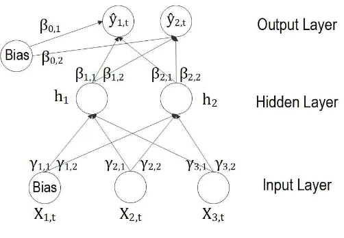
in-formation moves forward from a layer to the next one. Assuming a single hidden layer
[image:6.595.174.425.416.590.2]architecture, a FNN with multiple outputs can be depicted as in Figure 1.
Figure 1:FNN with two target variables, a single hidden layer with two hidden nodes and
three input variables (including the bias)
The output function of thek-th target variable, withk=1, . . . ,l(wherelis the number of target variables, e.g.l=2 in Figure 1), for FNN with a single hidden layer can be specified
as follows:
ˆ
yk,t=F¡
β0,k+ q
X
j=1 G¡
xtγ′j¢βj,k
¢
, (4)
whereGis the hidden layer activation function,βj,kis the weight from the j-th hidden unit
to the output unit,xt=
n
1,x1,t, . . . ,xs,t
o
m=s+1),β0,kis the bias of thek-th output unit,γj=
n
γ1,j, . . . ,γm,j
o
is the vector of weights
of dimension 1×mconnecting the input variables and the j-th hidden neuron andqis the number of hidden units.
Generally,F is an identity activation function, such thatF(a)=a. Equation (4) takes then the following form:
ˆ
yk,t=β0,k+ q
X
j=1 G¡
xtγ′j¢βj,k. (5)
In order to replicate the activation state of a biological neuron, all neural networks use
non-linear activation functions at some point, usually throughG. An ideal activation function
should be continuous and differentiable to implement the backpropagation algorithm. The
most common choices are a logistic and a hyperbolic tangent function.
The logistic cumulative function is bounded between 0 and 1, where a value closer to 0
(1) equals to a low (high) activation level, and can be specified as
G(x)= 1
1+e−x.
The hyperbolic tangent function is better suited for variables that assume negative values
and is bounded between -1 and 1. It can be written as
G(x)=e
x−e−x ex+e−x.
Both the functions have been used in the present work.
An interesting feature of biological neural networks is the presence of internal feedback.
Such feedback has been implemented in recurrent neural networks (RNN), where the
infor-mation is propagated from a layer to the succeeding layer but also back to earlier layers. In
this way, RNNs allow to preserve long-memory of time series and capture long-term
depen-dence with a restrained number of parameters. Therefore, in practical applications RNNs
are more appropriate than FNN to forecast nonlinear time series.
This analysis relies on four different types of recurrent neural networks: Elman, Jordan,
long short-term memory (LSTM) network and nonlinear autoregressive exogenous (NARX)
neural network.
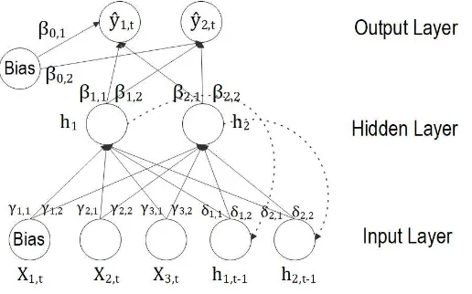
In an Elman neural network, introduced by Elman (1990), the hidden nodes with a time
delay are used as additional input neurons. Assuming an identity output function and a
single lag for the hidden nodes, the output of the Elman network with multiple outputs can
be represented as in Figure 2 and can be written as follows
ˆ
yk,t=β0,k+ q
X
j=1
ht j=G¡xtγ′j+ht−1δ′j¢ j=1, . . . ,q
whereht−1 is the vector of lagged hidden units and δj is the vector of connection weights
[image:8.595.172.430.231.392.2]between the j-th hidden node and the lagged hidden nodes.
Figure 2: ENN with a single hidden layer
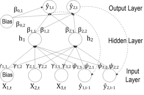
An alternative way to implement internal feedback is specifying a Jordan neural
net-work (JNN), proposed by Jordan (1986). As shown in Figure 3, a JNN exhibits a feedback
from the output to the input layer. The lagged output units are then used as additional
neurons. The way the output units are fed back has similarities with GARCH models,
mak-ing JNN an appetible way to forecast conditional volatility. Accordmak-ingly, the output of the
Jordan neural network (JNN) with multiple target variables can be computed as
ˆ
yk,t=β0,k+ q
X
j=1 G¡
xtγ′j+
l
X
k=1
ˆ
yk,t−1ψj,k
¢
βj,k (7)
whereψj,k is the weight between the lagged output and the j-th hidden unit for the target
Figure 3: JNN with a single hidden layer
Elman and Jordan neural networks, because of the presence of internal feedbacks, are
capable of detecting long-range relations. For this reason, such models have many potential
applications in economics and finance, see Kuan and Liu (1995) and Tino, Schittenkopf, and
Dorffner (2001).
Although traditional RNNs are able to model and forecast nonlinear time series with
great accuracy, they present several pitfalls. On one side, time lags of internal feedbacks
should be pre-determined by the researcher. On the other side, RNNs still suffer from the
presence of the vanishing gradient problem1. To overcome these issues, two further ways
to define nonlinear and persistent relationships through neural networks can be specified,
namely the NARX neural network and the long short-term memory (LSTM) neural network.
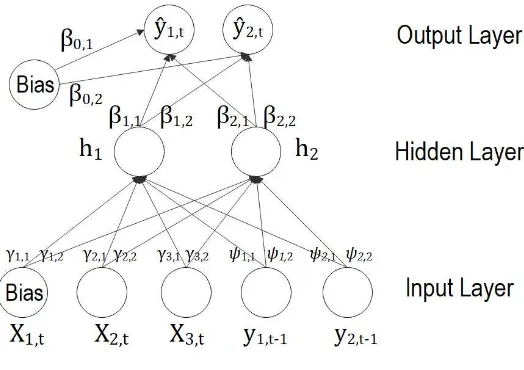
NARX neural network can be seen as an augmented version of FNN or JNN. In fact, it
allows to directly include lagged observed target variables or predicted output in the input
layer. In doing so, direct connections from the past mitigate the vanishing gradient problem
and capture long-term dependence.
There exist two ways to specify a NARX network:
• NARX-P, through a parallel (P) specification the predicted output units at timet are used as additional inputs in a FNN architecture at timet+1, similarly to a JNN;
1The vanishing gradient problem occurs when neural networks are trained through a gradient based
• NARX-SP, through a semi-parallel (SP) specificationdlags of the real target variables are included in the set of explanatory variables in the input layer. This architecture
behaves like a FNN where the input units are enriched by lagged observed outputs.
Throughout this paper, I will consider only a NARX-SP architecture with zero input
or-der and a multi-dimensional output, as depicted as in Figure 4. The output of this network
can be specified as follows:
yk,t=β0,k+ q
X
j=1 G¡
xtγ′j+ l
X
k nd X
d
yk,t−dψk,d,j
¢
βj,k (8)
[image:10.595.169.431.350.535.2]whereψk,d,jis the connection weight of thed-th delay of output unitk.
Figure 4:Architecture of a NARX network
The aforementioned recurrent neural networks are not the only architectures able to
replicate the way biological neurons remember through the internal feedback. In fact, the
most successful RNN to capture long-term dependencies is the long short-term memory
net-work (LSTM), proposed by Hochreiter and Schmidhuber (1997). The structure of a LSTM
is similar to other RNNs with an input layer, a recurrent hidden layer and an output layer.
However, in order to retain relevant information and to discard unnecessary parts, the
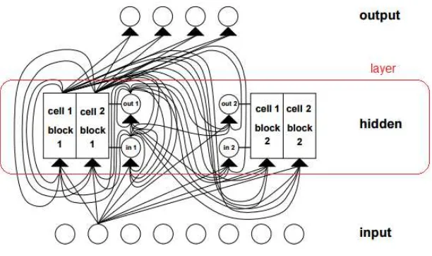
hid-den nodes are replaced by a memory block (see Figure 5), where a mechanism of gating
Figure 5: LSTM neural network
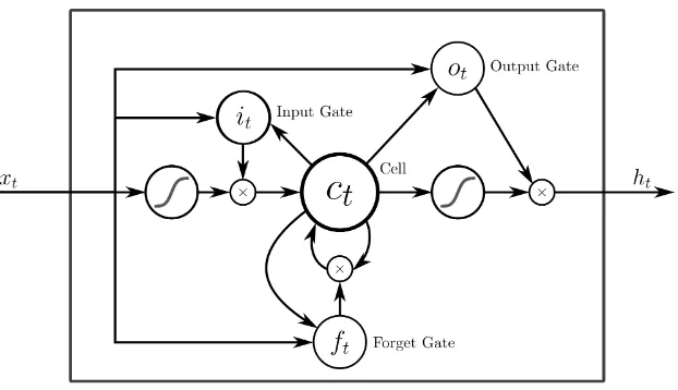
As depicted in Figure 6, each memory block is a self-connected system of three gates:
input, forget and output. Compared to traditional RNNs, a forget gate is added to the
memory block to prevent the gradient from vanishing or exploding, see also Hsu (2017). The
gating mechanism allows the network to learn which information should be maintained
and which not. The structure of a LSTM network with multiple target variables can be
formalized as below:
fk,t=G¡Wk,fhk,t−1+Uk,fxt+bk,f¢ (9)
ik,t=G¡Wk,ihk,t−1+Uk,ixt+bk,i¢ (10)
˜
ck,t=C¡Wk,chk,t−1+Uk,cxt+bk,c¢ (11)
ck,t=fk,t⊙ck,t−1+ik,t⊙c˜k,t (12)
ok,t=G¡Wk,ohk,t−1+Uk,oxt+Vk,ock,t+bk,o¢ (13)
hk,t=ok,t⊙C¡ck,t¢ (14)
ˆ
yk,t=hk,t (15)
whereWi,Wf,Wc,Wo,Ui,Uf,UcandUoare the weight matrices of input, forget, memory
cell state, and output gates respectively,Vc is the cell state weight matrix, ˆyk,t is thek-th
output of the neural network,bi, bf, bc and bo are the biases of each gate,G is a sigmoid
Figure 6: Basic LSTM memory block
LSTM is particularly useful, among others, in situations where the time series exhibits
a highly persistent behavior. For such reasons, it has been broadly applied in financial
studies, like Xiong, Nichols, and Shen (2016), Bao, Yue, and Rao (2017) and Kim and Won
(2018).
All the aforementioned types of neural networks are used to produce forecasts of the
Cholesky elements ofCt. Once the forecast of the lower triangular matrix, ˆCt+k, has been
obtained, the forecast realized covariance matrix can be re-constructed as
RCt+k=Cˆt+kCˆ′t+k,
ensuring a positive definite forecast of the covariance matrix, forn<Nt.
3
Neural Networks Architecture
When specifying a neural network architecture, the researcher should identify the set of
explanatory variables used as inputs, define the number of hidden layers and hidden nodes,
and choose the activation function and the training algorithm for the definition of the
con-nection weights.
The set of determinants is usually gathered from the related literature. From an
see Schwert (1989), Mele (2007), Paye (2012) and Christiansen, Schmeling, and Schrimpf
(2012). Here, the most part of the candidates as explanatory variables is based on excess
return predictability determinants. Following Mele (2007) and Welch and Goyal (2008), I
include in the analysis the dividend-price (DP) and the price-earnings ratio (EP), the equity
market return (MKT) and the Fama and French (1993) factors (HML, SMB and STR), which
typically influence risk premium. Since the set of independent variables include the returns
of two bond Futures, also the 1-month T-Bill rate (TB) and the term spread difference (TS)
between long-term and short-term bond yields are used as additional inputs. As in
Schw-ert (1989) and Engle, Ghysels, and Sohn (2009), the set of predictors is also enriched by
macroeconomic variables, as inflation rate (INF) and industrial production growth (IP).
Fi-nally, the default spread has been included as a proxy for the credit risk. All the exogenous
variables have been lagged one time to alleviate the endogeneity problem.
The definition of the number of hidden nodes and layers is more complicated. In fact,
there is no theoretical basis to determine the appropriate number of hidden layers or
neu-rons in a network. According to other studies and to the guidelines provided by Xiang, Ding,
and Lee (2005), a single-hidden layer architecture is sufficient to approximate a wide range
of nonlinear functions. Thus, in this paper a single hidden layer has been implemented.
Conversely, a poor number of hidden units does not allow to detect complex nonlinear
pat-terns in the data. However, when too many hidden units are included in the architecture,
the network may lead to overfitted out-of-sample forecasts and the number of connection
weights may significantly increase. In order to select the optimum number of weights, I
compare the sum of the RMSE for different architecture where the number of hidden nodes
varies from 1 to 8, as suggested by Tang and Fishwick (1993). Similarly to nonlinear
esti-mation techniques, the risk of a local minimum is high also for neural networks. In fact, the
training procedure is sensitive to the initial values of the weights randomly selected. To
as-sess the performance of the network, the parameters have been trained with 300 different
starting values. Since the architecture of a LSTM is significantly different from the rest of
the neural networks, a number of 100 memory blocks is chosen in line with similar works.
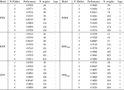
As shown in Table 1, a different number of hidden nodes provides very different results
in terms of cumulated RMSE. For FNN, the measure of performance is lower for a number
of hidden neurons equal to 5. ENN, ENN with lagged target variables and NARX network
exhibit the best performance when 3 hidden nodes are used, while JNN and JNN with lags
seem to forecast better with 6 and 2 hidden nodes, respectively.
lo-cal minimum could be significant. Accordingly, the connection weights have been trained
with a gradient descent with momentum and adaptive learning rate (gdx) algorithm for
all the networks, except for the NARX neural network. In fact, the NARX network has
been trained with a Bayesian Regularization (BR) algorithm, which allows to obtain robust
forecasts with a NARX network, as suggested by Guzman, Paz, and Tagert (2017).
Finally, all the activation functions, G, in Equation (4), (6), (7) and (8), are logistic
[image:14.595.91.519.343.653.2]functions.
Table 1: RMSE for increasing number of hidden nodes
The number of hidden neurons, the cumulated RMSE of themseries, the number of connection weights and the delays of the dependent variables used as inputs are included in the table. The maximum number of iterations is equal to 1000. ENNlags
and JNNlagsare ENN and JNN with lagged target variables as additional inputs. The training sample is approximately equal
to the 70% of the whole sample (from May 2007 to December 2017), while the testing sample is equal to 128 observations.
Model N. Hidden Performance N. weights Lags Model N. Hidden Performance N. weights Lags
FNN
1 0.0762 24
-NARX
1 0.0640 30 1
2 0.0771 42 - 2 0.0564 54 1
3 0.0732 60 - 3 0.0521* 78 1
4 0.0727 78 - 4 0.0561 102 1
5 0.0674* 96 - 5 0.0560 126 1
6 0.0686 114 - 6 0.0550 150 1
7 0.0698 132 - 7 0.0575 174 1
8 0.0709 150 - 8 0.0574 198 1
ENN
1 0.0743 25
-ENNlags
1 0.0739 31 1
2 0.0706 46 - 2 0.0729 58 1
3 0.0652* 69 - 3 0.0666* 87 1
4 0.0708 94 - 4 0.0718 118 1
5 0.0743 121 - 5 0.0776 151 1
6 0.0751 150 - 6 0.0866 186 1
7 0.0759 181 - 7 0.0845 223 1
8 0.0911 214 - 8 0.0865 262 1
JNN
1 0.0763 30
-JNNlags
1 0.0735 36 1
2 0.0769 54 - 2 0.0648* 66 1
3 0.0720 78 - 3 0.0667 96 1
4 0.0665 102 - 4 0.0657 126 1
5 0.0690 126 - 5 0.0668 156 1
6 0.0646* 150 - 6 0.0693 186 1
7 0.0682 174 - 7 0.0672 216 1
8 0.0696 198 - 8 0.0725 246 1
4
Empirical Results
The realized covariance matrices are computed according to Equation (1) and are based on
the daily returns on the S&P 500, on the 10-year Treasury note future and on the 1-month
Treasury bond future, both traded on the Chicago Board of Trade (CBOT)2. Thus, there are
T=428 monthly realized covariance matrices.
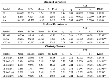
Table 2 shows summary statistics for the realized volatility and co-volatility series, and
for the Cholesky factors of the covariance matrices. The volatility of stock market is much
larger than average volatility of treasury futures. As is well known, realized variances
and covariances are highly persistent for stock market, as shown by the autocorrelation
coefficients.
The series of the Cholesky factors preserve the persistence exhibited by the original
covariance series, as suggested by Andersen and Bollerslev (1997) and Andersen, Bollerslev,
Diebold, and Ebens (2001), while unit root tests provide mixed results on the hypothesis of
stationary series. As proved by the skewness and the excess kurtosis of the time series, the
distribution of the Cholesky factors is far from being normal, for this reason a method free
from distribution assumptions, such as neural networks, could provide improved forecasts.
2Future contracts provide two major advantages: they are highly liquid and they permits to define bond
Table 2: Descriptive statistics Realized Covariance and Cholesky factors series
The table includes the mean, the standard deviation, skewness, excess kurtosis and the sample autocorrelation. The last three columns report thep-value of the Dickey-Fuller (ADF) with constant (c) and with constant and trend (c-t) and the KPSS test statistics.
Realized Variances
ADF
Symbol Mean St.Dev Skew. Ex. Kurt. ρ1 ρ2 c c-t KPSS
SP 25.526 50.284 8.54 95.36 0.44 0.31 0.0000 0.0000 0.1099 10Y 4.135 6.927 13.46 229.6 0.11 0.10 0.0000 0.0000 0.5813∗∗ 1m 10.190 17.739 14.16 242.9 0.09 0.07 0.0000 0.0000 0.1201
Realized Covariances
ADF
Symbol Mean St.Dev. Skew. Ex. Kurt. ρ1 ρ2 c c-t KPSS
SP-10Y -0.090 5.616 -1.164 12.22 0.55 0.41 <0.001 <0.001 1.9393∗∗∗ SP-1m -0.284 9.218 -0.829 8.500 0.57 0.42 <0.001 <0.001 2.0829∗∗∗ 10Y-1m 6.023 10.667 15.22 275.9 0.08 0.08 <0.001 <0.001 0.4254∗
Cholesky Factors
ADF
Symbol Mean St.Dev. Skew. Ex. Kurt. ρ1 ρ2 c c-t KPSS
Cholesky 1 4.338 2.592 3.46 19.68 0.63 0.52 <0.001 <0.001 0.1433 Cholesky 2 0.124 0.899 0.13 0.246 0.70 0.67 0.075 <0.001 2.5495∗∗∗ Cholesky 3 1.633 0.805 4.81 48.06 0.38 0.24 0.031 <0.001 0.8056∗∗∗ Cholesky 4 0.149 1.457 -0.03 -0.09 0.72 0.71 0.206 <0.001 2.6791∗∗∗ Cholesky 5 2.380 1.149 6.48 81.03 0.31 0.27 <0.001 <0.001 0.3891∗ Cholesky 6 0.823 0.626 9.87 149.5 0.26 0.24 <0.001 <0.001 0.5334∗∗ Where: *** -p-value < 1% , ** -p-value < 5%, * -p-value < 10%
The aim of the paper is to produce more accurate forecasts than existing econometric
models in a multivariate context. To this end, time series were first divided in an in-sample
set, from May 1982 to April 2007, and an out-of-sample set, from May 2007 to December
2017 (128 monthly observations), which equals to third of the whole sample. The
one-step-ahead out-of-sample forecasts from the neural networks model are compared with the
forecasts from a Cholesky-VAR (Vector Autoregressive) model with and without predictors,
a VAR on the original realized covariance matrices, and a DCC model.
The evaluation of the out-of-sample forecasts is a crucial aspect for the choice of the
model best fitting the data. Common problems arising in the comparison of volatility
fore-casts concern the latent nature of the target variable and the choice of an adequate loss
function. The former issue has been addressed by using a volatility proxy, such as realized
volatility. Thus, throughout the paper volatility is assumed as observable. In regard to
the latter, Patton (2011) provided the necessary and sufficient conditions for a loss
func-tion. Based on these conditions, the loss function here used are the MSE loss function for
univariate comparison, and Frobenius distance between matrices and Euclidean distance
between vectors for multivariate comparison, such that
LMSE=( ˆσt−ht)2
LF( ˆΣt,Ht)=∥Σˆt−Ht∥2F
LE( ˆσt,ht)=vech( ˆΣt−Ht)′vech( ˆΣt−Ht)
where ˆσt is the single element of the volatility matrix proxy, ˆΣt, while ht is the single
element of the variance matrix forecast,Ht.
The performance is evaluated for each element of the covariance matrices through Mean
Absolute Error (MAE), the Root Mean Squared Error (RMSE) and through the equal
pre-dictive accuracy test by Diebold and Mariano (1995) (DM). The DM test is also performed
in the multivariate framework through the multivariate loss functions above mentioned.
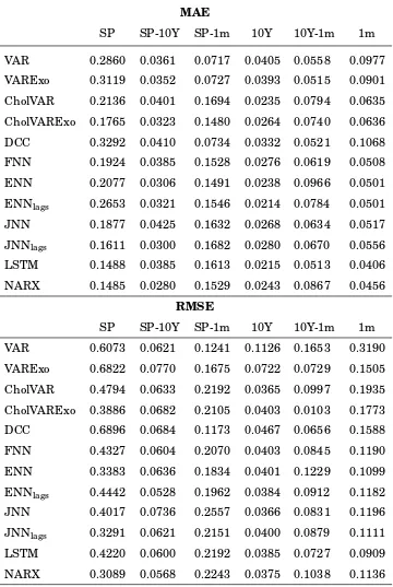
In Table 3, the accuracy measures are computed for each covariance series. For several
realized covariances, MAE and RMSE are minimum for the NARX and the LSTM neural
networks. Not surprisingly, neural networks provide overall better results than linear
mod-els for the majority of the series. Moreover, the use of the Cholesky decomposition seems to
improve the out-of-sample forecasting accuracy.
The DM tests for the single elements of the covariance matrices have been computed
using the forecasts from the VAR model without exogenous variables as benchmark model.
model performs worse than the compared model. In the most of the pairwise comparison
in Table 4, the loss difference is positive but almost never significant. Recurrent neural
networks are able to outperform VAR model only in forecasting the realized variance of S&P
500, while the test provides not significant loss differences for all the other time series.
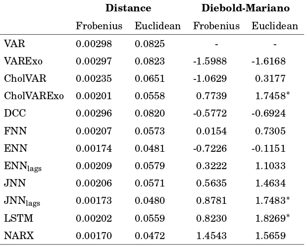
Additionally, DM test has been conducted on multivariate loss function differences, as
shown in Table 5, together with the error measured with Frobenius and Euclidean
dis-tances. VAR, VARExo and DCC exhibit the highest error among the compared models.
The best performance is shown by the JNN with lagged target variables and NARX
mod-els, underlying the relevance of detecting long-term persistence with an adequate
archi-tecture. When considering the DM on multivariate loss functions, the test statistics is
positively significant only when Euclidean norm is applied and only for three models: VAR
on Cholesky factors with exogenous variables, JNN with lagged realized covariances as
in-puts and LSTM. In the multivariate context, NARX is able to outperform all the competing
models, except for the DM-Euclidean statistics.
When looking at each single element of the covariance matrices,only minor gains are
found from using neural networks in forecasting realized covariances. In a multivariate
context, the choice of the forecasting method seems to slightly affect the forecasting
ac-curacy if a single target variable is considered. Conversely, there is evidence that the
re-current neural networks, especially LSTM and NARX networks, provide the best realized
covariance forecasts when the whole set of forecasts is evaluated. Interestingly, neural
net-works are shown to be particularly useful to forecast highly persistent series, once again
underlying the relevance of an approach suited for detecting long-term dependencies.
A reason why neural networks cannot outperform competing models in this context can
be found in the presence of unit roots in several Cholesky factor series, such asCholesky 2,
Cholesky 3andCholesky 4, on which the networks are trained. Furthermore, the lack of a
significant difference in the forecasting accuracy with econometric models can be dictated
by the large number of parameters respect to the number of observations, which may lead
Table 3: Out-of-sample Forecasts Evaluation
MAE
SP SP-10Y SP-1m 10Y 10Y-1m 1m
VAR 0.2860 0.0361 0.0717 0.0405 0.0558 0.0977 VARExo 0.3119 0.0352 0.0727 0.0393 0.0515 0.0901 CholVAR 0.2136 0.0401 0.1694 0.0235 0.0794 0.0635 CholVARExo 0.1765 0.0323 0.1480 0.0264 0.0740 0.0636 DCC 0.3292 0.0410 0.0734 0.0332 0.0521 0.1068 FNN 0.1924 0.0385 0.1528 0.0276 0.0619 0.0508 ENN 0.2077 0.0306 0.1491 0.0238 0.0966 0.0501 ENNlags 0.2653 0.0321 0.1546 0.0214 0.0784 0.0501 JNN 0.1877 0.0425 0.1632 0.0268 0.0634 0.0517 JNNlags 0.1611 0.0300 0.1682 0.0280 0.0670 0.0556 LSTM 0.1488 0.0385 0.1613 0.0215 0.0513 0.0406 NARX 0.1485 0.0280 0.1529 0.0243 0.0867 0.0456
RMSE
SP SP-10Y SP-1m 10Y 10Y-1m 1m
VAR 0.6073 0.0621 0.1241 0.1126 0.1653 0.3190 VARExo 0.6822 0.0770 0.1675 0.0722 0.0729 0.1505 CholVAR 0.4794 0.0633 0.2192 0.0365 0.0997 0.1935 CholVARExo 0.3886 0.0682 0.2105 0.0403 0.0103 0.1773 DCC 0.6896 0.0684 0.1173 0.0467 0.0656 0.1588 FNN 0.4327 0.0604 0.2070 0.0403 0.0845 0.1190 ENN 0.3383 0.0636 0.1834 0.0401 0.1229 0.1099 ENNlags 0.4442 0.0528 0.1962 0.0384 0.0912 0.1182 JNN 0.4017 0.0736 0.2557 0.0366 0.0831 0.1196 JNNlags 0.3291 0.0621 0.2151 0.0400 0.0879 0.1111 LSTM 0.4220 0.0600 0.2192 0.0385 0.0727 0.0909 NARX 0.3089 0.0568 0.2243 0.0375 0.1038 0.1136
Table 4: Diebold-Mariano test - MSE Loss Function
SP SP-10Y SP-1m 10Y 10Y-1m 1m
VARExo -0.6309 -0.8942 -1.0472 0.6589 0.8982 0.9178
CholVAR 1.4217 -0.3653 -4.8336∗∗∗ 1.0301 0.7108 1.0532
CholVARExo 1.7873∗ -0.8061 -3.3350∗∗∗ 1.0123 0.7099 1.0283
DCC -0.8045 -1.1784 0.3256 0.9517 0.9403 0.8879
FNN 1.3850 0.3362 -3.4702∗∗∗ 1.0028 0.8234 1.0168
ENN 1.6905∗ -0.1670 -3.0251∗∗∗ 1.0039 0.4957 1.0410
ENNlags 1.4462 1.9721∗ -3.3147∗∗∗ 1.0167 0.7759 1.0230
JNN 1.6830 -1.0598 -3.2517∗∗∗ 1.0288 0.8332 1.0149
JNNlags 1.9081∗ 0.0013 -3.6584∗∗∗ 1.0052 0.7994 1.0382
LSTM 1.8202∗ 0.4082 -3.5759∗∗∗ 1.0158 0.8995 1.0853
NARX 1.8647∗ 1.1590 -3.2338∗∗∗ 1.0239 0.6771 1.0326
Table 5: Statistical Evaluation with Multivariate Loss Functions
Distance Diebold-Mariano
Frobenius Euclidean Frobenius Euclidean
VAR 0.00298 0.0825 -
-VARExo 0.00297 0.0823 -1.5988 -1.6168
CholVAR 0.00235 0.0651 -1.0629 0.3177
CholVARExo 0.00201 0.0558 0.7739 1.7458∗
DCC 0.00296 0.0820 -0.5772 -0.6924
FNN 0.00207 0.0573 0.0154 0.7305
ENN 0.00174 0.0481 -0.7226 -0.1151
ENNlags 0.00209 0.0579 0.3222 1.1033
JNN 0.00206 0.0571 0.5635 1.4634
JNNlags 0.00173 0.0480 0.8781 1.7483∗
LSTM 0.00202 0.0559 0.8230 1.8269∗
[image:20.595.145.455.426.675.2]5
Conclusions
This study represents the first attempt to model multivariate volatility through artificial
neural networks, in order to detect nonlinear dynamics and long-term dependencies in the
realized covariance series. The use of such models allows to detect possible nonlinear
re-lationships without the a priori knowledge of the distribution of the variables at a
signif-icantly reduced computational effort. However, this approach is not costless, since with
an increasing number of hidden layers and hidden nodes the number of parameters to be
trained and the risk of a local minimum increase rapidly.
The main purpose of the paper is to understand whether the use of the Cholesky
de-composition combined with the implementation of neural networks, specifically recurrent
neural networks, is able to outperform traditional econometric method in forecasting
re-alized covariance matrices. At this end, the out-of-sample forecasting accuracy of a set of
neural networks is compared with existing econometric methods.
Several conclusions emerge from the statistical evaluation of the out-of-sample
fore-casts. First, contrary to the literature on univariate models, NNs show a modest gain in
forecasting accuracy when applied to multivariate persistent time series. Second, long-term
dependence detecting models, like NARX and LSTM, seem to provide the best forecasting
performance, as underlined by the comparison through multivariate loss functions.
Moreover, the use of the Cholesky decomposition seems to improve the forecasting
accu-racy respect to models which are not based on a parametrization, like the VAR, the VARExo
and the DCC model.
Future works could implement different parametrizations of the realized covariance
matrices, like the logarithmic transformation used by Bauer and Vorkink (2011). A further
analysis could rely on different input variables and different target variables, like the
ex-change rate volatility or the crude oil volatility. Another interesting application would be
References
ANDERSEN, T. G., AND T. BOLLERSLEV(1997): “Heterogeneous information arrivals and return volatility dynamics: Uncovering the long-run in high frequency returns,”Journal
of Finance, 52, 975–1005.
ANDERSEN, T. G., T. BOLLERSLEV, F. X. DIEBOLD, ANDH. EBENS (2001): “The distribu-tion of realized stock return volatility,”Journal of Financial Economics, 61, 43–76.
ANDERSEN, T. G., T. BOLLERSLEV, F. X. DIEBOLD,ANDP. LABYS(2001): “The distribution of exchange rate volatility,”Journal of American Statistical Association, 96, 42–55.
(2003): “Modeling and Forecasting Realized Volatility,”Econometrica, 71, 579–625.
ANDERSON, H. M., K. NAM,ANDF. VAHID(1999): Asymmetric Nonlinear Smooth
Transi-tion Garch Modelspp. 191–207. Springer US.
BAO, W., H. YUE,ANDY. RAO(2017): “A deep learning framework for financial time series using stacked autoencoders and long-short term memory,”PLoS One, 12(7).
BARNDORFF-NIELSEN, O. E.,ANDN. SHEPHARD(2002): “Estimating Quadratic Variation
Using Realised Variance,”Journal of Applied Econometrics, 17, 457–477.
(2004): “Power and Bipower Variation with Stochastic Volatility and Jumps,” Jour-nal of Financial Econometrics, 2, 1–37.
BAUER, G. H., AND K. VORKINK(2011): “Forecasting multivariate realized stock market volatility,”Journal of Econometrics, 160, 93–101.
BECKER, R., A. CLEMENTS, AND R. O’NEILL(2010): “A Cholesky-MIDAS model for pre-dicting stock portfolio volatility,” Working paper, Centre for Growth and Business Cycle
Research Discussion Paper Series.
BUCCI, A. (2019): “Realized Volatility Forecasting with Neural Networks,” Working paper.
BUCCI, A., G. PALOMBA, AND E. ROSSI(2019): “Does macroeconomics help in predicting
stock market volatility comovements? A nonlinear approach,” Working paper.
CHRISTIANSEN, C., M. SCHMELING, AND A. SCHRIMPF(2012): “A comprehensive look at financial volatility prediction by economic variables,” Journal of Applied Econometrics,
DIEBOLD, F. X., AND R. S. MARIANO (1995): “Comparing predictive accuracy,”Journal of Business and Economic Statistics, 13, 253–263.
DONALDSON, G. R.,ANDM. KAMSTRA(1997): “An artificial neural network-GARCH model
for international stock return volatility,”Journal of Empirical Finance, 4, 17–46.
ELMAN, J. L. (1990): “Finding structure in time,”Cognitive Science, 14(2), 179–211.
ENGLE, R. F., E. GHYSELS, AND B. SOHN (2009): “On the Economic Sources of Stock
Market Volatility,” Working paper.
FAMA, E., AND K. FRENCH (1993): “Common Risk Factors in the Returns on Stocks and Bonds,”Journal of Financial Economics, 33, 3–56.
FERNANDES, M., M. C. MEDEIROS, AND M. SCHARTH (2014): “Modeling and predicting the CBOE market volatility index,”Journal of Banking & Finance, 40, 1–10.
GUZMAN, S. M., J. O. PAZ, AND M. L. M. TAGERT (2017): “The Use of NARX Neural
Networks to Forecast Daily Groundwater Levels,”Water Resour Manage, 31, 1591–1603.
HALBLEIB-CHIRIAC, R., AND V. VOEV (2011): “Modelling and Forecasting Multivariate Realized Volatility,”Journal of Applied Econometrics, 26, 922–947.
HEIDEN, M. D. (2015): “Pitfalls of the Cholesky decomposition for forecasting multivariate volatility,” Working paper.
HOCHREITER, S.,AND J. SCHMIDHUBER (1997): “Long short-term memory,”Neural Com-putation, 9(8), 1735–1780.
HSU, D. (2017): “Time Series Forecasting Based on Augmented Long Short-Term Memory,”
Working paper.
HU, Y. M., AND C. TSOUKALAS (1999): “Combining conditional volatility forecasts using neural networks: an application to the EMS exchange rates,” Journal of International
Financial Markets, Institutions & Money, 9, 407–422.
JORDAN, M. I. (1986): “Serial Order: A Parallel Distributed Processing Approach,”
KHAN, A. I. (2011): “Financial Volatility Forecasting by Nonlinear Support Vector Machine Heterogeneous Autoregressive Model: Evidence from Nikkei 225 Stock Index,”
Interna-tional Journal of Economics and Finance, 3(4), 138–150.
KIM, H. Y., AND C. H. WON(2018): “Forecasting the volatility of stock price index: A hy-brid model integrating LSTM with multiple GARCH-type models,”Expert Systems with
Applications, 103, 25–37.
KUAN, C.,ANDT. LIU(1995): “Forecasting exchange rates using feedforward and recurrent
neural networks,”Journal of Applied Econometrics, 10(4), 347–364.
KWAN, C., W. LI,ANDK. NG(2005): “A Multivariate Threshold GARCH Model with Time-varying Correlations,” Working Paper.
MAHEU, J. M., AND T. H. MCCURDY (2002): “Nonlinear features of realized volatility,”
Review of Economics and Statistics, 84, 668–681.
MARTENS, M., M. DE POOTER, AND D. J. VAN DIJK (2004): “Modeling and Forecasting
S&P 500 Volatility: Long Memory, Structural Breaks and Nonlinearity,” Tinbergen
Insti-tute Discussion Paper No. 04-067/4.
MELE, A. (2007): “Asymmetric stock market volatility and the cyclical behavior of expected returns,”Journal of Financial Economics, 86, 446–478.
PATTON, A. J. (2011): “Volatility forecast comparison using imperfect volatility proxies,”
Journal of Econometrics, 160(1), 246 – 256.
PAYE, B. S. (2012): “Dèjà vol: Predictive regressions for aggregate stock market volatility using macroeconomic variables,”Journal of Financial Economics, 106, 527–546.
SCHWERT, W. G. (1989): “Why does stock market volatility change over time,”Journal of Finance, 44, 1115–1153.
TANG, Z., AND P. A. FISHWICK (1993): “Feed-forward Neural Nets as Models for Time Series Forecasting,”ORSA Journal on Computing, 5, 374–385.
TINO, P., C. SCHITTENKOPF,ANDG. DORFFNER(2001): “Financial volatility trading using
VORTELINOS, D. I. (2017): “Forecasting realized volatility: HAR against Principal Compo-nents Combining, neural networks and GARCH,”Research in International Business and
Finance, 39, 824–839.
WELCH, I., AND A. GOYAL (2008): “A comprehensive look at the empirical performance of equity premium prediction,”Review of Financial Studies, 21(4), 1455–1508.
WHITE, H. (1988): Economic prediction using neural networks: the case of IBM daily stock returns. IEEE 1988 International Conference on Neural Networks.
XIANG, C., S. DING, AND T. H. LEE (2005): “Geometrical interpretation and architecture
selection of MLP,”IEEE Transactions on Neural Networks, 16(1), 84–96.
