Second Order Semantic Dependency Parsing with End to End Neural Networks

4609

Second-Order Semantic Dependency Parsing with End-to-End Neural

Networks

Xinyu Wang, Jingxian Huang, Kewei Tu∗

School of Information Science and Technology, ShanghaiTech University, Shanghai, China

{wangxy1,huangjx,tukw}@shanghaitech.edu.cn

Abstract

Semantic dependency parsing aims to iden-tify semantic relationships between words in a sentence that form a graph. In this paper, we propose a second-order semantic depen-dency parser, which takes into consideration not only individual dependency edges but also interactions between pairs of edges. We show that second-order parsing can be approximated using mean field (MF) variational inference or loopy belief propagation (LBP). We can unfold both algorithms as recurrent layers of a neural network and therefore can train the parser in an end-to-end manner. Our experi-ments show that our approach achieves state-of-the-art performance.

1 Introduction

Semantic dependency parsing (Oepen et al.) aims to produce graph-structured semantic depen-dency representations of sentences instead of tree-structured syntactic dependency parses. Exist-ing approaches to semantic dependency parsExist-ing can be classified as graph-based approaches and transition-based approaches. In this paper, we investigate graph-based approaches which score each possible parse of a sentence by factorizing over its parts and search for the highest-scoring parse.

Previous work in graph-based syntactic depen-dency parsing has shown that higher-order pars-ing generally outperforms first-order parspars-ing ( Mc-Donald and Pereira, 2006; Carreras, 2007; Koo and Collins, 2010; Ma and Zhao, 2012). While a first-order parser scores dependency edges in-dependently, a higher-order parser takes relation-ships between two or more edges into considera-tion. However, most of the previous algorithms for higher-order syntactic dependency tree pars-ing are not applicable to semantic dependency

∗_{Corresponding Author}

graphparsing, and designing efficient algorithms for higher-order semantic dependency graph pars-ing is nontrivial. In addition, it becomes a com-mon practice to use neural networks to compute features and scores of parse graph components, which ideally requires backpropagation of parsing errors through the higher-order parsing algorithm, adding to the difficulty of designing such an algo-rithm.

In this paper, we propose a novel graph-based second-order semantic dependency parser. Given an input sentence, we use a neural network to com-pute scores for both first and second-order parts of parse graphs and then apply either mean field variational inference or loopy belief propagation to approximately find the highest-scoring parse graph. Both algorithms are iterative inference al-gorithms and we show that they can be unfolded as recurrent layers of a neural network with each layer representing the computation in one itera-tion of the algorithms. In this way, we can con-struct an end-to-end neural network that takes in a sentence and outputs the approximate marginal probability of every possible dependency edge. During training, we maximize the probability of the gold parses by using standard gradient-based methods. Our experiments show that our approach achieves state-of-the-art performance in semantic dependency parsing and outperforms our baseline with 0.3% and 0.4% labeled F1 score and previ-ous state-of-the-art model with 1.3% and 1.4% la-beled F1 score for in-domain and out-of-domain test sets respectively. Our approach shows more advantage over the baseline when there are fewer training data and when parsing longer sentences.

2 Semantic Dependency Parsing

Embedding

BiLSTM FNN

Biaffine or Trilinear Function

MF/LBP Recurrent Layers

Edge Prediction

Label Prediction Q(#)

…

Q(%)

s('()')

[s(+,-)_{; s}()/)_{; s}(01/)_]

h_,('()'−4/()

h_,(67-'6−4/()

89

8:

;9

;:

h_<('()'−4/()

h_<(67-'6−4/() s(67-'6) h_,(+,-); h_,()/); h_,(01/)

h_<(+,-); h_<()/); h_<(01/)

Figure 1: Illustration of our model architecture.

et al.) aiming at recovering semantic dependency relationships in sentences of the WSJ corpus. It was extended in SemEval-2015 task 18 (Oepen et al., 2015) with an additional out-of-domain dataset (the Brown corpus). A semantic dency parse is different from a syntactic depen-dency parse in that the dependepen-dency edges are an-notated with semantic relations (e.g., agent and pa-tient) and form a directed acyclic graph instead of a tree. The Broad-Coverage Semantic Depen-dency Parsing provides three different formalisms:

DM,PASandPSD. Previous work has found that PAS is the easiest to learn and PSD is the most difficult as it has the largest set of labels.

3 Approach

Our model architecture (shown in Figure 1) fol-lows that ofDozat and Manning(2018). Given an input sentence, we first compute word representa-tions using a BiLSTM, which are then fed into two parallel modules, one for predicting the existence of every edge and the other for predicting the label of every edge. The label-prediction module makes predictions of each edge independently and hence is a first-order decoder. The edge-prediction mod-ule is what our approach differs from that ofDozat and Manning(2018). The module scores both first and second-order parts and then goes through mul-tiple recurrent inference layers to predict edge ex-istence.

3.1 Part Scoring

Given a sentence with n words [w1, w2, ..., wn], we feed a BiLSTM with their word embeddings and POS tag embeddings.

oi=e(word)i ⊕e

(postag)

i

R= BiLSTM(O)

whereoi is the concatenation (⊕) of the word and POS tag embeddings of word wi, O represents

[o1, . . . ,on], andR = [r1, . . . ,rn]represents the output from the BiLSTM.

To score first-order parts (edges) in both the edge-prediction module and the label-prediction module, we use two single-layer feedforward net-works (FNNs) to compute a head representation and adependentrepresentation for each word and then apply a biaffine function to compute the scores of edges and labels.

Biaff(v1,v2) :=vT1Uv2+b

h(edge-head)_i =FNN(edge-head)(ri)

h(edge-dep)_i =FNN(edge-dep)(ri)

h(label-head)_i =FNN(label-head)(ri)

h(label-dep)_i =FNN(label-dep)(ri)

s(edge)_ij = Biaff(edge)(h(edge-dep)_i ,h(edge-head)_j ) (1)

s(label)_ij = Biaff(label)_(h(label-dep)

i ,h

(label-head)

j ) (2)

In Eq. 2, the tensorU in the biaffine function is

p a1 a2 a p1 p2 g p a

grandparent siblings co-parents

Figure 2: Second-order parts used in our model.

i6=j,ui,c,j = 0), wheredis hidden size andcis the number of labels. In Eq.1, the tensorUin the biaffine function isd×1×d-dimensional.

In the edge-prediction module, we further score second-order parts. We consider three types of second-order parts: siblings (sib), co-parents (cop) and grandparents (gp) (Martins and Almeida,

2014), as shown in Figure2. For a specifictype

of second-order part, we use single-layer FNNs to compute a head representation and a dependent representation for each word. For grandparent parts, we additionally compute ahead_dep repre-sentation for each word.

type∈ {sib, cop, gp}

h(_itype-head)=FNN(type-head)(ri)

h(_itype-dep)=FNN(type-dep)(ri)

h(gp-head_dep)_i =FNN(gp-head_dep)(ri)

We then apply a trilinear function to compute scores of second-order parts. A trilinear function is defined as follows.

Trilin(v1,v2,v3) :=vT3vT1Uv2

whereUis a(d×d×d)-dimensional tensor. To reduce the computation cost, we assume that U has rank d and can be represented as the prod-uct of three(d×d)-dimensional matricesU1,U2

andU3. We can then compute second-order part

scores as follows.

gi:=Uivi i∈[1,2,3]

Trilin(v1,v2,v3) :=

d

X

i=1

g1i◦g2i◦g3i (3)

s(_ij,iksib)≡s(_ik,ijsib)= Trilin(sib)(h(head)_i ,h(dep)_j ,h(dep)_k )

(4)

s(_ij,kjcop)≡s(_kj,ijcop)= Trilin(cop)(h(head)_i ,h(dep)_j ,h(head)_k )

(5)

s(_ij,jkgp) = Trilin(gp)(h_i(head),h(head_dep)_j ,h(dep)_k )

(6)

where◦represents element-wise product. We re-quirej < kin Eq. 4andi < kin Eq.5.

<TOP> 0

They 1

were 2

not 3

Poles 4

Sibling factor Co-parent factor

Grandparent factor Unary factor

1,3 3,1 2,4 4,2

0,2 0,3

0,4

0,1 1,2 2,1

1,4 4,1

2,3 3,2 3,4 4,3

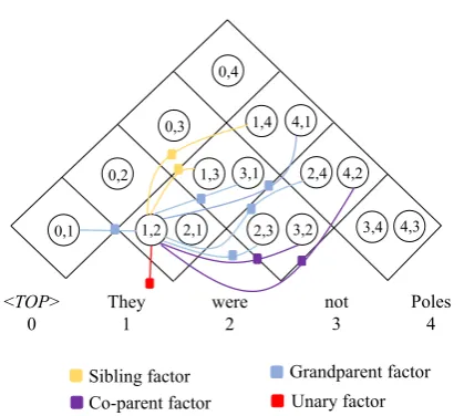
Figure 3: An example of our factor graph for a sentence with four words. The node <TOP> is the top of de-pendency graph. The boolean variable(i, j)indicates whether the directed edge(i, j)exists. For simplicity, we only depict factors connected to node(1,2).

3.2 Inference

In the label-prediction module,s(label)_i,j is fed into a softmax layer that outputs the probability of each label for edge(i, j). In the edge-prediction mod-ule, computing the edge probabilities can be seen as doing posterior inference on a Conditional Ran-dom Field (CRF). The corresponding factor graph is shown in Figure3. Each Boolean variableXijin the CRF indicate whether the directed edge(i, j)

exists. We use Eq. 1to define our unary potential

ψu representing scores of an edge and Eqs. (4

-6) to define our binary potentialψp. We define a unary potentialφu(Xij)for each variableXij.

φu(Xij) =

(

exp(s(edge)_ij ) Xij = 1

1 Xij = 0

For each pair of edges(i, j)and(k, l)that form a second-order part of a specifictype, we define a binary potentialφp(Xij, Xkl).

φp(Xij, Xkl) =

(

exp(s(_ij,kltype)) Xij =Xkl= 1

0 Otherwise

every edge(i, j)such thatQij(1)>0.5. The edge labels are predicted by maximizing the label prob-abilities computed by the label-prediction module.

Mean Field Variational Inference

Mean field variational inference approximates a true posterior distribution with a factorized vari-ational distribution and tries to iteratively mini-mize their KL divergence. We can derive the fol-lowing iterative update equations of distribution

Qij(Xij).

F_ij(t−1) = X

k6=i,j

Q(_ikt−1)(1)s(_ij,iksib)+Q(_kjt−1)(1)s(_ij,kjcop)

+Q(_jkt−1)(1)s(_ij,jkgp) +Q(_kit−1)(1)s(_ki,ijgp)

(7)

Q(_ijt)(0)∝1

Q(_ijt)(1)∝exp{s(edge)_ij +F_ij(t−1)}

The initial distributionQ(0)_ij (Xij)is set by normal-izing the unary potentialφu(Xij). We iteratively update the distributions forT steps and then out-putQ(_ijT)(Xij), whereT is a hyperparameter.

Loopy Belief Propagation

Loopy belief propagation iteratively passes mes-sages between variables and potential functions (factors). Because our CRF contains only unary and binary potentials, we can merge each variable-to-factor message and its subsequent factor-to-variable message into a single factor-to-variable-to-factor-to-variable messageMkl→ij, representing message from edge

(k, l) to edge (i, j). The update function of the messages in each iteration is:

Q(_ijt−1)(Xij) =φu(Xij)

Y

ab∈Nij

M_ab(t−_→1)_ij(Xij)

M_kl(t_→) _ij(0)∝X xkl

Q_kl(t−1)(xkl)/Mij(t→−1)kl(xkl)

M_kl(t_→) _ij(1)∝Q_kl(t−1)(0)/M_ij(t_→−1)_kl(0)

+ exp(s(_ij,kltype))Q_kl(t−1)(1)/M_ij(t_→−1)_kl(1)

We initialize the messages withM_kl(0)_→ij = 1. We iteratively update the messages and distributions forT steps and then outputQ(_ijT)(Xij).

Inference as Recurrent Layers

Zheng et al.(2015) proposed that a fixed number of iterations in mean field variational inference can be seen as a recurrent neural network that is pa-rameterized by the potential functions. We follow

the idea and unfold both mean field variational in-ference and loopy belief propagation as recurrent neural network layers that are parameterized by part scores.

The time complexity of our inference procedure is O(n3), which is lower than the O(n4) com-plexity of the exact quasi-second-order inference ofCao et al.(2017) and on par with the complex-ity of the approximate second-order inference of

Martins and Almeida(2014).

3.3 Learning

Given a gold parse graph y⋆ _{of sentence w, the} conditional distribution over possible edgey_ij(edge)

and corresponding possible label y(label)_ij is given by:

P(y(edge)_ij |w) =softmax(Q(_ijT)(Xij))

P(y_ij(label)|w) =softmax(s(label)_ij )

We define the following cross entropy losses:

L(edge)(θ) =−X

i,j

log(Pθ(y_ij⋆(edge)|w))

L(label)(θ) =−X

i,j

✶(y⋆_ij(edge)) log(Pθ(y⋆ij(label)|w))

whereθis the parameters of our model,✶(y⋆_ij(edge))

denotes the indicator function and equals 1 when edge (i, j) exists in the gold parse and 0 other-wise, andi, jranges over all the words in the sen-tence. We optimize the weighted average of the two losses.

L=λL(label)+ (1−λ)L(edge)

whereλis a hyperparameter.

4 Experiments

4.1 Hyperparameters

We tuned the hyperparameters of our baseline model from Dozat and Manning (2018) and our second-order model on the DM development set. We followed Dozat and Manning (2018) using 100-dimensional pretrained GloVe embeddings (Pennington et al.,2014) and transformed them to be 125-dimensional. Words and lemmas appeared less than 7 times are replaced with a special un-known token. We use the same dataset split as in previous approaches (Martins and Almeida,2014;

Hidden Layer Hidden Sizes

Word/Glove/Lemma/Char 100

POS 50

GloVe Linear 125

BiLSTM LSTM 3*600

Char LSTM 1*400

Unary Arc/Label 600

Binary Arc 150

Dropouts Dropout Prob.

Word/GloVe/POS/Lemma 20%

Char LSTM (FF/recur) 33%

Char Linear 33%

BiLSTM (FF/recur) 45%/25%

Unary Arc/Label 25%/33%

Binary Arc 25%

Optimizer & Loss Value Baseline Interpolation (λ) 0.025 Second-Order Interpolation (λ) 0.07

Adamβ1 0

Adamβ2 0.95

Learning rate 1_e−2

LR decay 0.5

L2 regularization (MF/LBP) 3_e−9

/3_e−8

Weight Initialization Mean/Stddev

Unary weight (Eq.1) 0.0/1.0

Binary weight (Eq.3) 0.0/0.25

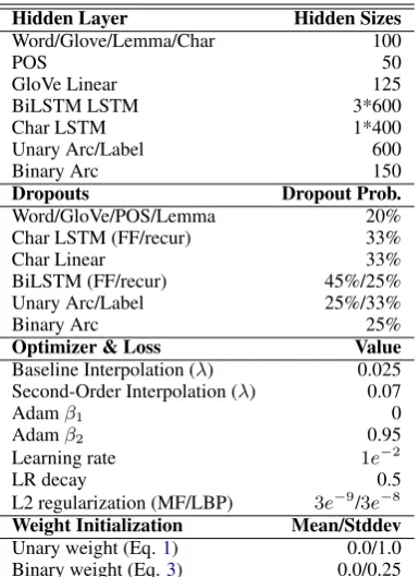
Table 1: Hyperparameter for baseline and second-order models in our experiment.

1,410 sentences in the in-domain test set and 1,849 Brown Corpus sentences in the out-of-domain test set. We additionally removed sentences longer than 60 in order to speed up training, which re-sults in 33,916 training sentences. The final hy-perparameters of our baseline and second-order model are shown in Table 1. Following Dozat and Manning(2018), we used Adam (Kingma and Ba,2014) for optimizing our model, annealing the learning rate by 0.5 for every 10,000 steps, and switched the optimizer to AMSGrad (Reddi et al.,

2018) after 5,000 steps without improvement. We trained the model for 100,000 iterations with batch sizes of 6,000 tokens and terminated training early after 10,000 iterations with no improvement on the development sets.

4.2 Main Results

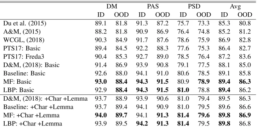
We compare our model with previous state-of-the-art approaches in Table 2. Du et al. (2015) is a hybrid model. A&M is fromAlmeida and Martins

(2015).PTS17proposed by (Peng et al.,2017) and Basicis single task parsing whileFreda3is a mul-titask parser across three formalisms. WCGL18 (Wang et al., 2018) is a neural transition-based model. D&M (Dozat and Manning, 2018) is a graph-based model and "Baseline" is the

first-order model fromDozat and Manning(2018) that was trained by ourselves. For our model, we used mean field variational inference and loopy belief propagation for 3 iterations.

In the basic setting, on average our model out-performs the best previous one by1.3%on the in-domain test set and1.3%on the out-of-domain test set. With lemma and character-based embeddings, our model leads to an average improvement of

0.3%and0.6%over previous models. Our model also outperforms the baseline by0.2%− −0.5%

on average with different settings and test sets.

Dozat and Manning(2018) found that on the PAS dataset their model cannot benefit from lemma and character-based embeddings and hence speculated that they may have approached the ceiling of the PAS F1 score. As shown in our experiments on the PAS dataset, our model cannot benefit from lemma and character-based embeddings either, but it obtains higher F1 scores, which suggests that the ceiling may not have been reached.

Note that while we do not force our parser to predict a directed acyclic graph, we found that only 0.7% of the test sentences have cycles in their parses.

4.3 Analysis

Small Training Data

To evaluate the performance of our model on smaller training data, we repeated our experiments with randomly sampled 70%, 40% and 10% of the training set. Table3shows the F1 scores averaged over 5 runs (each time with a new randomly sam-pled training subset). It can be seen that the advan-tage of our model over the baseline increases sig-nificantly when the training data becomes smaller. We make the following speculation to explain this observation. The BiLSTM layer in the baseline and our model is capable of capturing high-order information to some extent. However, without prior knowledge of high-order parts, it may require more training data to learn this capability than a high-order decoder. So with small training data, the baseline loses the capability of utilizing high-order information, while our model can still rely on the decoder for high-order parsing.

Performance on Different Sentence Lengths

DM PAS PSD Avg

ID OOD ID OOD ID OOD ID OOD

Du et al. (2015) 89.1 81.8 91.3 87.2 75.7 73.3 85.3 80.8

A&M, (2015) 88.2 81.8 90.9 86.9 76.4 74.8 85.2 81.2

WCGL, (2018) 90.3 84.9 91.7 87.6 78.6 75.9 86.9 82.8

PTS17: Basic 89.4 84.5 92.2 88.3 77.6 75.3 86.4 82.7

PTS17: Freda3 90.4 85.3 92.7 89.0 78.5 76.4 87.2 83.6

D&M, (2018): Basic 91.4 86.9 93.9 90.8 79.1 77.5 88.1 85.0

Baseline: Basic 92.6 88.0 94.1 91.0 80.6 78.5 89.1 85.8

MF: Basic 93.0 88.4 94.3 91.5 80.9 78.9 89.4 86.3

LBP: Basic 92.9 88.4 94.3 91.5 81.0 78.8 89.4 86.2

D&M, (2018): +Char +Lemma 93.7 88.9 93.9 90.6 81.0 79.4 89.5 86.3

Baseline: +Char +Lemma 93.7 89.4 94.1 90.9 81.0 79.5 89.6 86.6

MF: +Char +Lemma 94.0 89.7 94.1 91.3 81.4 79.6 89.8 86.9

LBP: +Char +Lemma 93.9 89.5 94.2 91.3 81.4 79.5 89.8 86.8

Table 2: Comparison of labeled F1 scores achieved by our model and previous state-of-the-arts. The F1 scores of Baseline and our models are averaged over 5 runs. ID denotes the in-domain (WSJ) test set and OOD denotes the out-of-domain (Brown) test set. +Char and +Lemma means augmenting the token embeddings with character-level and lemma embeddings.

DM PAS PSD Avg

ID OOD ID OOD ID OOD ID OOD

Baseline: 70% 92.0 87.0 93.8 90.6 79.8 77.7 88.5 85.1

MF: 70% 92.4 87.5 93.9 90.8 80.2 78.0 88.8 85.4

LBP: 70% 92.3 87.4 94.0 90.9 80.2 78.1 88.8 85.5

Baseline: 40% 90.8 85.5 93.2 89.6 78.4 76.4 87.4 83.8

MF: 40% 91.2 86.0 93.4 90.0 78.9 76.7 87.8 84.2

LBP: 40% 91.2 86.0 93.5 90.0 78.9 76.8 87.9 84.3

Baseline: 10% 86.1 80.0 90.8 86.4 73.5 71.2 83.4 79.2

MF: 10% 86.9 81.0 91.3 87.1 74.5 72.1 84.2 80.1

LBP: 10% 86.8 80.9 91.3 87.0 74.5 72.3 84.2 80.1

Table 3: Comparison of labeled F1 scores achieved by our model and our baseline on 10%, 40%, 70% of the training data. We report the average F1 score over 5 runs with different randomly sampled training data.

and evaluate our model and the baseline on them. Figure 4 shows that our model has more advan-tage over the baseline when sentences get longer, especially when sentences are longer than 40. One possible explanation is that BiLSTM has difficulty in capturing long-range dependencies in long sen-tences, which leads to lower performance on the first-order baseline; but such long-range depen-dencies can still be captured with second-order parsing. It can also be seen that on long sen-tences, our model has more advantage over the baseline for the out-of-domain test set than for the in-domain test set, which suggests that our model has better generalizability especially on long sen-tences.

Mean Field vs. Loopy Belief Propagation

We compare mean field variational inference and loopy belief propagation algorithms in Table 4. We tuned the hyperparameters of our model for each algorithm and iteration number separately. We find that in general mean field variational in-ference has very similar performance to loopy be-lief propagation. In addition, with more iterations, the performance of mean field variational infer-ence steadily increases while the at the second it-eration.

Ablation Study

0-10 10-20 20-30 30-40

40-0 0.5 1

In-Domain

Labeled

F1

Dif

ference

MF%10 MF%40

MF%70 MF%100

LBP%10 LBP%40

LBP%70 LBP%100

0-10 10-20 20-30 30-40

40-0 0.5 1 1.5 2

Out-of-Domain

Labeled

F1

Dif

ference

MF%10 MF%40

MF%70 MF%100

LBP%10 LBP%40

LBP%70 LBP%100

Figure 4: Relative improvements over our baseline in different sentence length intervals with different training data sizes. We report the average F1 score improvements over all the formalisms with 5 runs for each.

Iteration ID OOD

MF

1 92.78 88.38

2 92.86 88.37

3 92.98 88.44

LBP

1 92.88 88.29

2 92.84 88.17

3 92.88 88.36

Table 4: Comparison of labeled F1 scores of mean field and loopy belief propagation with different iteration numbers on the DM dataset.

ID OOD

Baseline 92.60 87.98

+Siblings 92.85 88.31

+Co-parents 92.80 88.23

+Grandparents 92.84 88.24

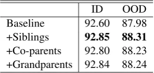
Table 5: The performance comparison between three types of second-order parts on the DM dataset.

type of second-order parts without the other two types on the DM dataset using mean field varia-tional inference and the result is shown in Table5. While all the three types of second-order parts can be seen to improve the parsing performance over the baseline, the sibling parts lead to the largest performance gain on both the in-domain test set and the out-of-domain test set.

4.4 Case Study

We provide a parsing example in Figure5to show how our second-order parser with 3 iterations of

mean field variational inference works. Before the first iteration, the marginal distributions of edges

Qij is initialized with unary potentials and thus is exactly what a first-order parser would pro-duce. In the subsequent iterations, the distribu-tions are updated with binary potentials taken into account. For each version of the distributions, we can extract a parse graph by collecting edges with probabilities larger than 0.5. From Figure 5, we can see that erroneous edges are gradually fixed through iterations. Edge (were, P oles) sends a strong negative co-parents message to edge

(<T OP>, P oles)in the first iteration, so the latter has a lower probability in subsequent iterations. Edge(were, P oles) also sends a strong positive grandparent message to edge(<T OP>, were) to enhance its probability, and the latter sends an increasingly positive message back to the for-mer in subsequent iterations. In the second and third iterations,(were, P oles)sends positive sib-ling messages and(<T OP>, were)sends positive grandparent messages to enhance probabilities of edges (were, T hey) and (were, not), which fi-nally leads to the correct parse.

4.5 Running Speed

Our model have a time complexity ofO(d2

u+d2b+

n3)while the first order model ofDozat and Man-ning(2018) has a time complexity ofO(d2_u+n2)

<TOP>

They

were

not

Poles

They were not Poles

(1) 1st iteration

<TOP>

They

were

not

Poles

They were not Poles

(2) 2nd iteration

<TOP>

They

were

not

Poles

They were not Poles

(3) 3rd iteration

<TOP>

They

were

not

Poles

They were not Poles

(4) Final prediction

They were not Poles

<TOP> <TOP>

(1) 1st iteration

They were not Poles

<TOP>

(2) 2nd iteration

They were not Poles

<TOP>

(3) 3rd iteration

They were not Poles

<TOP>

(4) Final prediction

Figure 5: An example of message passing (left) and the corresponding graph parses (right) in our second-order parser with mean field variational inference. We regard terms in Eq. 7as messages sent from other arcs. Blue arcs and red arcs on the left represent positive messages (whichencouragethe target edge to exist) and negative messages (whichdiscouragethe target edge to exist) respectively. Lightness of the arc color represents the message intensity. Blackness of each nodes represents the probability of edge existence. A Node with a double circle means the corresponding edge is predicted to exist. Messages with low intensities are omitted in the graph. Dotted arcs and red arcs on the right represent missed predictions and wrong predictions compared to the golden parse. The period in the sentence is omitted for simplicity.

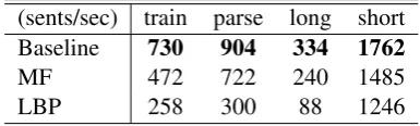
(sents/sec) train parse long short

Baseline 730 904 334 1762

MF 472 722 240 1485

LBP 258 300 88 1246

Table 6: Training and parsing speed (sentences/second) comparison of the baseline and our model (3 iterations for our second-order parser). long means the parsing speed on sentences longer than 40 andshortmeans the parsing speed on sentences no longer than 10.

speed on an Nvidia Tesla P40 server. The result is shown in Table6. Mean field variational inference slows down training and parsing by 35% and 20% respectively compared with the baseline. How-ever, loopy belief propagation slows down training and parsing by 65% and 67% respectively com-pared with the baseline.

4.6 Significance Test

We trained 25 basic models of our approach and the baseline with the same hyperparameters in Table 1 on each formalism. Student’s t-test shows that our second-order model outperforms our baseline model on all the formalisms with a significance level of 0.005.

5 Related Work

5.1 Semantic Dependency Parsing

Semantic dependency parsing can be classified as transition-based approaches and graph-based approaches. Wang et al. (2018) proposed a transition-based parser for semantic parsing, while

et al. (2018) further proposed to learn from dif-ferent corpora. Dozat and Manning (2018) pro-posed a graph-based simple but powerful neural network for semantic dependency parsing using a bilinear or biaffine (Dozat and Manning,2016) layer to encode the interaction between words. Most of these approaches proposed first-order dependency parser while Martins and Almeida

(2014) proposed a way to encode higher-order parts with hand-crafted features and introduced a novel co-parent part for semantic dependency parsing. They used discrete optimizing algorithm alternating directions dual decomposition (AD3) as their decoder. Cao et al. (2017) also proposed a quasi-second-order semantic dependency parser

with dynamic programming. Our model

con-tains second-order information comparing with the first-order approaches and benefits from end-to-end training comparing with other second-order approaches.

5.2 Higher-Order Dependency Parsing

Higher-order parsing has been extensively studied in the literature of syntactic dependency parsing. Much of these work is based on the first-order maximum spanning tree (MST) parser of McDon-ald et al. (2005) which factorizes a dependency tree into individual edges and maximizes the sum-mation of the scores of all the edges in a tree. Mc-Donald and Pereira (2006) introduced a second-order MST that factorizes a dependency tree into not only edges but also second-order sibling parts, which allows interactions between adjacent sib-ling words. Carreras(2007) defined second-order grandparent parts representing grandparental rela-tions. Koo and Collins (2010) introduced third-order sibling and tri-sibling parts. A grand-sibling part represents a grandparent with two grandchildren and a tri-sibling part represents a parent with three children. Ma and Zhao(2012) defined grand-tri-sibling parts for fourth-order de-pendency parsing.

Many previous approaches to higher-order de-pendency parsing perform exact decoding based on dynamic programming, but there is also re-search in approximate higher-order parsing. Mar-tins et al. (2011) proposed an alternating direc-tions dual decomposition (AD3) algorithm which splits the original problem into several local sub-problems and solves them iteratively. They em-ployed AD3 for second-order dependency parsing

to speed up decoding. Smith and Eisner (2008) andGormley et al. (2015) proposed to use belief propagation for approximate higher-order parsing, which is closely related to our work.

While higher-order parsing has been shown to improve syntactic dependency parsing accuracy, it receives less attention in semantic dependency parsing. Martins and Almeida (2014) proposed second-order semantic dependency parsing and employed AD3 for approximate decoding. Cao et al.(2017) proposed a quasi-second-order parser and used dynamic programming for decoding with time complexity ofO(n4).

5.3 CRF as Recurrent Neural Networks

Zheng et al.(2015) are probably the first to pro-pose the idea of unfolding iterative inference al-gorithms on CRFs as a stack of recurrent neural network layers. They unfolded mean field varia-tional inference in a neural network designed for semantic segmentation. There is a lot of subse-quent work that employs this technique, especially in the computer vision area. For example, Zhu et al.(2017) proposed a structured attention neural model for Visual Question Answering with a CRF over image regions and unfolded both mean field variational inference and loopy belief propagation algorithms as recurrent layers.

6 Conclusion

We proposed a novel graph-based second-order parser for semantic dependency parsing. We constructed an end-to-end neural network that uses a trilinear function to score second-order parts and finds the highest-scoring parse graph by either mean field variational inference or loopy belief propagation algorithms unfolded as recurrent neural network layers. Our exper-imental results show that our model outper-forms previous state-of-the-art model and has higher accuracies especially on out-of-domain

data and long sentences. Our code is

pub-licly available at https://github.com/

wangxinyu0922/Second_Order_SDP

Acknowledgments

References

Mariana SC Almeida and André FT Martins. 2015. Lisbon: Evaluating turbosemanticparser on multiple languages and out-of-domain data. InProceedings of the 9th International Workshop on Semantic Eval-uation (SemEval 2015), pages 970–973.

Junjie Cao, Sheng Huang, Weiwei Sun, and Xiao-jun Wan. 2017. Quasi-second-order parsing for 1-endpoint-crossing, pagenumber-2 graphs. In Pro-ceedings of the 2017 Conference on Empirical Meth-ods in Natural Language Processing, pages 24–34.

Xavier Carreras. 2007. Experiments with a higher-order projective dependency parser. InProceedings of the 2007 Joint Conference on Empirical Methods in Natural Language Processing and Computational Natural Language Learning (EMNLP-CoNLL).

Timothy Dozat and Christopher D Manning. 2016. Deep biaffine attention for neural dependency pars-ing. arXiv preprint arXiv:1611.01734.

Timothy Dozat and Christopher D Manning. 2018. Simpler but more accurate semantic dependency parsing.arXiv preprint arXiv:1807.01396.

Yantao Du, Fan Zhang, Xun Zhang, Weiwei Sun, and Xiaojun Wan. 2015. Peking: Building semantic de-pendency graphs with a hybrid parser. In Proceed-ings of the 9th international workshop on semantic evaluation (semeval 2015), pages 927–931.

Matthew R Gormley, Mark Dredze, and Jason Eisner. 2015. Approximation-aware dependency parsing by belief propagation. Transactions of the Association for Computational Linguistics, 3:489–501.

Diederik P Kingma and Jimmy Ba. 2014. Adam: A method for stochastic optimization. arXiv preprint arXiv:1412.6980.

Terry Koo and Michael Collins. 2010. Efficient third-order dependency parsers. In Proceedings of the 48th Annual Meeting of the Association for Com-putational Linguistics, pages 1–11. Association for Computational Linguistics.

Xuezhe Ma and Hai Zhao. 2012. Fourth-order de-pendency parsing. Proceedings of COLING 2012: posters, pages 785–796.

André FT Martins and Mariana SC Almeida. 2014. Priberam: A turbo semantic parser with second or-der features. InProceedings of the 8th International Workshop on Semantic Evaluation (SemEval 2014), pages 471–476.

André FT Martins, Noah A Smith, Pedro MQ Aguiar, and Mário AT Figueiredo. 2011. Dual decomposi-tion with many overlapping components. In Pro-ceedings of the Conference on Empirical Methods in Natural Language Processing, pages 238–249. As-sociation for Computational Linguistics.

Ryan McDonald, Koby Crammer, and Fernando Pereira. 2005. Online large-margin training of de-pendency parsers. In Proceedings of the 43rd An-nual Meeting of the Association for Computational Linguistics (ACL’05), pages 91–98.

Ryan McDonald and Fernando Pereira. 2006. Online learning of approximate dependency parsing algo-rithms. In11th Conference of the European Chapter of the Association for Computational Linguistics.

Stephan Oepen, Marco Kuhlmann, Yusuke Miyao, Daniel Zeman, Silvie Cinková, Dan Flickinger, Jan Hajic, and Zdenka Uresova. 2015. Semeval 2015 task 18: Broad-coverage semantic dependency pars-ing. InProceedings of the 9th International Work-shop on Semantic Evaluation (SemEval 2015), pages 915–926.

Stephan Oepen, Marco Kuhlmann, Yusuke Miyao, Daniel Zeman, Dan Flickinger, Jan Hajic, Angelina Ivanova, and Yi Zhang. Semeval 2014 task 8: Broad-coverage semantic dependency parsing.

Hao Peng, Sam Thomson, and Noah A Smith. 2017. Deep multitask learning for semantic dependency parsing.arXiv preprint arXiv:1704.06855.

Hao Peng, Sam Thomson, Swabha Swayamdipta, and Noah A Smith. 2018. Learning joint se-mantic parsers from disjoint data. arXiv preprint arXiv:1804.05990.

Jeffrey Pennington, Richard Socher, and Christopher Manning. 2014. Glove: Global vectors for word representation. InProceedings of the 2014 confer-ence on empirical methods in natural language pro-cessing (EMNLP), pages 1532–1543.

Sashank J Reddi, Satyen Kale, and Sanjiv Kumar. 2018. On the convergence of adam and beyond.

David A Smith and Jason Eisner. 2008. Dependency parsing by belief propagation. InProceedings of the Conference on Empirical Methods in Natural Lan-guage Processing, pages 145–156. Association for Computational Linguistics.

Yuxuan Wang, Wanxiang Che, Jiang Guo, and Ting Liu. 2018. A neural transition-based approach for semantic dependency graph parsing. In Thirty-Second AAAI Conference on Artificial Intelligence.

Shuai Zheng, Sadeep Jayasumana, Bernardino Romera-Paredes, Vibhav Vineet, Zhizhong Su, Dalong Du, Chang Huang, and Philip HS Torr. 2015. Conditional random fields as recurrent neural networks. InProceedings of the IEEE international conference on computer vision, pages 1529–1537.