Cross Validating Synthetic Controls

Munich Personal RePEc Archive

Cross-Validating Synthetic Controls

Becker, Martin and Klößner, Stefan and Pfeifer, Gregor

Saarland University, Saarland University, University of Hohenheim

17 August 2017

Online at

https://mpra.ub.uni-muenchen.de/83679/

Cross-Validating Synthetic Controls

Martin Becker, Saarland University

Stefan Kl¨oßner, Saarland University

Gregor Pfeifer, University of Hohenheim

October 12, 2017

Abstract

While the literature on synthetic control methods mostly abstracts from out-of-sample measures, Abadie et al. (2015) have recently introduced a cross-validation approach. This

technique, however, is not well-defined since it hinges on predictor weights which are not uniquely defined. We fix this issue, proposing a new, well-defined cross-validation

technique, which we apply to the original Abadie et al. (2015) data. Additionally, we discuss how this new technique can be used for comparing different specifications based

on out-of-sample measures, avoiding the danger of cherry-picking.

JEL Codes: C52, C22

Keywords: Synthetic Control Methods; Cross-Validation; Specification Search.

∗_{Corresponding author: Stefan Kl¨oßner, Statistics & Econometrics, Saarland University, C3 1, D-66123,}

1

Introduction

Abadie and Gardeazabal (2003) and Abadie et al. (2010) have introduced synthetic control

methods (SCM) to estimate a treated unit’s development in absence of the treatment. These

methods have gained a lot of popularity among applied researchers, Athey and Imbens (2017)

even state that SCM “is arguably the most important innovation in the policy evaluation

literature in the last 15 years”. Recently, SCM have been shown to perform well against

certain panel-based approaches (see Gardeazabal and Vega-Bayo, 2017), and have also been

used for forecasting (see Kl¨oßner and Pfeifer, 2017).

The basic idea of SCM is to find suitable donor weights describing how the treated unit is

‘synthesized’ by a weighted mix of unaffected control units, building a counterfactual. Treated

and synthetic unit should resemble each other as closely as possible prior to the treatment,

both with respect to the outcome of interest and economic predictors. The latter are variables

with predictive power for explaining the outcome. The SCM approach searches for optimal

predictor weights in order to grant more importance to variables with better predictive power.

However, SCM operate merely in-sample, making it difficult to assess the counterfactual’s

validity. To mitigate this problem, Abadie et al. (2015) (henceforth: ADH) have expanded

SCM, incorporating cross-validation. The pre-treatment timespan is divided into a training

and a validation period, and predictor weights are selected by minimizing the out-of-sample

error in the validation period. However, Kl¨oßner et al. (2017) (henceforth: KKPS) have recently

shown that there is a misconception of the ADH cross-validation technique. In applications,

there often exist many different solutions that minimize the out-of-sample error, rendering this

technique not well-defined since predictor weights are not uniquely defined.

We fix this problem by defining unique predictor weights following two principles. Special

predictors like lagged values of the outcome variable(s) are guaranteed to obtain certain

mini-mum weights, and predictors in general shall not become irrelevant due to weights accidentally

obtained too small. Applying this new cross-validation technique to ADH’s original data, we

exemplarily show that ADH’s main finding is confirmed, while corresponding placebo exercises

F ir st st ep : ‘T rai n in g’

Donor weights in training period:

for any given predictor weights V, use predictor data

X₀(train), X₁(train)to determine ‘training’ donor weights

W∗

(train)(V), minimizing

||V12

X₁(train)−X₀(train)W

||2_.

Predictor weights by cross-validation:

use data on outcome,

Y₀(valid), Y₁(valid), to determine the setV _{of all predictor weights}V

minimizing ||Y₁(valid)−Y₀(valid)W∗

(train)(V)||2

and choose unique V∗_∈V_.

S ec on d st ep : ‘M ai n

’ _{Main donor weights:}

use predictor weightsV∗ _and

predictor dataX₀(valid), X₁(valid)

to determine main donor weights

W∗

(main)(V∗), minimizing

||V∗12

X₁(valid)−X₀(valid)W

||2_.

Counterfactual:

UseW∗

(main)(V∗)and

post-treatment values of outcome,Y₀(post), to calculate

b

Y₁(post):=Y₀(post)W∗

(main)(V∗).

Training Period Validation Period Post-Treatment

Period

Pre-Treatment Period

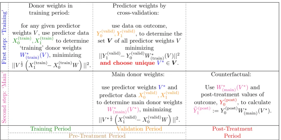
Figure 1: Schematic Overview of Cross-Validation Technique. This is a refined version of KKPS’s Figure 1.

2

SCM and Cross-Validation

For the synthetic control method, one uses two types of data—the variable of interest, Y, and

predictor variables, X. The latter consist of M linear combinations of pre-treatment values of

Y as well as r other covariates with explanatory power for Y. Both Y and X are considered

for a treated unit and for so-called donors, i.e., non-treated units, denoted by subscripts “1”

and “0”, respectively. In the example discussed by ADH and KKPS and also throughout this

paper, the treated unit is the 1990 reunified Germany, while (J = 16) Western OECD countries

serve as donors. The variable of interest (Y) is GDP per capita, and the k =M +r predictors

(X) are the average of lagged GDP values (M = 1) and the covariates trade openness, inflation

rate, industry share of value added, amount of schooling, and the investment rate (r= 5).1

The corresponding quantities as well as a schematic overview of the cross-validation

tech-nique are provided in Figure 1. The SCM cross-validation approach consists of two steps.

During the first step, called ’training’, so-called predictor weights V∗

are determined using

cross-validation techniques, during the second step, these weights V∗

are used to estimate the

variable of interest’s counterfactual development in absence of the treatment. For

determin-ing V∗

, the training step decomposes the pre-treatment timespan (1971-1990) into a training

(1971-1980) and a validation period (1981-1990). In the training period, one makes use of the

k×J matrix X₀(train)and thek-dimensional vectorX₁(train), containing time averages of the

pre-dictors’ data for the donor units and the treated unit, respectively. Given these, one considers,

for any given positive predictor weights V = (v1, . . . , vk)′ ∈Rk++, the so-called training weights

W∗

(train)(V)∈RJ, which are defined as the solution of

min W ||V

1 2

X₁(train)−X₀(train)W||2 = min W

k

X

m=1 vm

X₁(train)_m −X₀(train)_m W 2

s.t. W ≥0,✶′

W = 1,

(1)

whereV 12 is thek-dimensional diagonal matrix with the roots ofV’s elements on the diagonal,

while X₁(train)_m and X₀(train)_m denote the m-th component and row of X₁(train) and X₀(train),

respec-tively, and ✶ is the vector of ones. The training weights W∗

(train)(V) describe to what extent

each donor country is used during the training step to produce a ’synthetic’, i.e.,

counterfac-tual, Germany, given that the predictors are weighted according to V. As the training weights

W∗

(train)(V) depend on the predictor weights V, one aims at finding those predictor weights V

∗

that produce the best forecast. This is done in the second part of the training step, making

use of the data in the validation period, the L×J matrix Y₀(valid) and the L-dimensional

vec-tor Y₁(valid), containing the variable of interest’s data for the validation period. In particular,

ADH define predictor weights V∗

= (v∗

1, . . . , v

∗

k) as the predictor weights that minimize the out-of-sample error ||Y₁(valid)−Y₀(valid)W∗

(train)(V)||2 overV, i.e., V

∗ _{is the solution of}

min V ||Y

(valid) 1 −Y

(valid) 0 W

∗

(train)(V)||2 s.t. V ≥0,✶

′

V = 1, (2)

where the predictor weights, without loss of generality, have been normalized to sum to unity.

AfterV∗

has been determined, one proceeds to the ’main’ step, calculating the donor weights

W∗

(main)(V

∗

) as the minimizer of

min W

k

X

m=1 v∗

m

X₁(valid)_m −X₀(valid)_m W2 s.t. W ≥0,✶′

W = 1, (3)

where thek×J matrixX₀(valid) and thek-dimensional vectorX₁(valid) contain the predictors’ data

for the validation period. Eventually, counterfactual values Yb₁(post) for comparing with actual

valuesY₁(post)are given by Y₀(post)W∗

(main)(V

∗

), whereY₀(post)contains the donors’ post-treatment

However, KKPS show that this approach often leads to ambiguous counterfactual values

because V∗

is not well-defined due to Equation (2) not having a unique solution, but many

different minimizers:

V _{:={V :V is a minimizer of Equation (2)} (4)}

denotes the corresponding set of minimizers, which often is not a singleton. Thus, in order to

come up with a well-defined cross-validation technique, it is necessary to single out one specific,

uniquely defined element of V_{. In order to do so, we first prevent predictors related with the}

outcome from being attributed too small predictor weights, as otherwise the dependent variable

may be fitted very poorly in the ’main’ step. Therefore, we restrict V _to

e V _:=

      

V ∈V _:

1

M M

P

m=1 vm

max m=1,...,kvm

≥ 1

2maxev∈V 1

M M

P

m=1e vm

max m=1,...,kevm

      

,

ensuring that the outcome-related predictors’ relative importance must not fall below half

of what it could maximally be. Second, no economic predictor should accidentally become

essentially irrelevant due to an extremely small relative weight. Thus, within Ve_{, the ratio}

of the smallest over the largest predictor weight should be as large as possible, i.e., m=1min,...,kvm

max

m=1,...,kvm

should be maximal withinVe_{. If there exists more than one element of}Ve _{with that property, we}

can among those choose the one for which the ratio v(2)

max

m=1,...,kvm

of the second-smallest predictor

weight, v(2), over the largest predictor weight becomes maximal. If, again, there are several

solutions to this maximization problem, we may maximize among those the ratio v(3)

max

m=1,...,kvm

,

and so on. Proposition 1 in the appendix shows that this procedure results in uniquely defined

predictor weights V∗

.

3

Estimating the Effect of the German Reunification

Equipped with our new, properly defined cross-validation approach, we now compare the results

of ADH and KKPS to the results our new method delivers.2

The unique predictor weights delivered by our cross-validation technique are 80.94% for

2_{Calculations were done using the statistics software R-3.3.3 (see R Core Team, 2017) in combination with}

GDP per capita, 5.82% for trade openness, 1.11% for inflation, 1.11% for industry share of

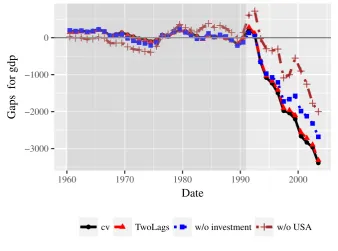
value added, 4.77% for amount of schooling, and 6.25% for investment rate. The corresponding

estimated gap due to the reunification, the difference between actual and counterfactual values,

is displayed in Figure 2 (black, solid line, labeled ’cv’). In line with ADH and KKPS, we

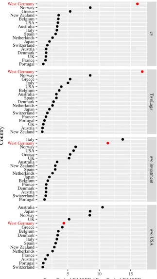
find a loss of ca. 3,000 USD. This loss is due to Germany’s reunification, as the upper part

of Figure 3 reveals, which shows the ratio of root mean squared differences between actual

and counterfactual GDP after and before the reunification for a so-called placebo study. Here,

each donor country is artificially assigned as the treated unit, while Germany moves to the

donor pool. The post-pre-ratio of Germany is much larger than all placebo countries’ ratios,

indicating that the measured loss in GDP can actually be considered statistically significant.

● ● ● ● ● ● ●

● ● ● ● ● ●●_{● ●}● ●● ● ● ●_{● ●●●●●●} ●●

● ●

●

● ●

●

● ● ●

● ●

●

●

−3000 −2000 −1000 0

1960 1970 1980 1990 2000

Date

Gaps for gdp

●

● _{cv TwoLags w/o investment w/o USA}

Figure 2: Gaps between GDP per capita of actual and synthetic Germany, estimated using cross-validation with specifications of ADH (’cv’), using last two outcome lags (’TwoLags’), without investment (’w/o investment’), and without U.S. data (’w/o USA’).

Our new cross-validation technique is also useful for comparing different specifications

ac-cording to an objective out-of-sample measure, without the danger of cherry-picking.3 _For

instance, instead of using the lagged outcomes’ average, one might choose the two most

re-cent lagged outcome values as predictors, as in Montalvo (2011). This specification performs

actually slightly better than ADH’s specification, with an RMSPE in the validation period of

65.616 compared to 67.678. As Figures 2 and 3 show, results for this specification are very

similar to those for ADH’s specification. Alternatively, when removing the investment rate

from the predictor set or excluding the U.S. from the donor pool, the cross-validation criterion

rises to 70.198 or 84.728, respectively. The corresponding timelines in Figure 2 still show a

considerable estimated loss in GDP per capita due to the reunification. However, estimated

losses are much smaller than for the other specifications, especially those derived without data

on the U.S. Correspondingly, Figure 3 shows that these reductions are no longer significant

according to the placebo study. When investment is discarded, Germany’s post-pre-ratio is

only the second-largest, while it is only the fifth-largest when the U.S. data are removed from

the sample. Thus, confirming the findings of KKPS and in contrast to ADH, we find that the

● ● ● ● ● ● ● ● ● ● ● ● ● ● ● ● ● ● ● ● ● ● ● ● ● ● ● ● ● ● ● ● ● ● ● ● ● ● ● ● ● ● ● ● ● ● ● ● ● ● ● ● ● ● ● ● ● ● ● ● ● ● ● ● ● ● ● cv T w oLags w/o in v estment w/o USA

5 10 15

West Germany USA UK Austria Belgium Denmark France Italy Netherlands Norway SwitzerlandJapan Greece Portugal Spain Australia New Zealand West Germany USA UK Austria Belgium Denmark France Italy Netherlands Norway SwitzerlandJapan Greece Portugal Spain Australia New Zealand West Germany USA UK Austria Belgium DenmarkFrance Italy Netherlands Norway Switzerland Japan Greece Portugal Spain Australia New Zealand

West GermanyUK

Austria Belgium Denmark France Italy Netherlands Norway Switzerland Japan Greece Portugal Spain Australia New Zealand

Post−Period RMSPE / Pre−Period RMSPE

Country

References

Abadie, A., Diamond, A., and Hainmueller, J. (2010). Synthetic Control Methods for Compar-ative Case Studies: Estimating the Effect of California’s Tobacco Control Program. Journal of the American Statistical Association, 105(490):493–505.

Abadie, A., Diamond, A., and Hainmueller, J. (2015). Comparative Politics and the Synthetic Control Method. American Journal of Political Science, 59(2):495–510.

Abadie, A. and Gardeazabal, J. (2003). The Economic Costs of Conflict: A Case Study of the

Basque Country. The American Economic Review, 93(1):113–132.

Athey, S. and Imbens, G. W. (2017). The state of applied econometrics: Causality and policy evaluation. Journal of Economic Perspectives, 31(2):3–32.

Becker, M. and Kl¨oßner, S. (2017a). Fast and Reliable Computation of Generalized Synthetic Controls. Econometrics and Statistics, pages n/a–n/a.

Becker, M. and Kl¨oßner, S. (2017b). MSCMT: Multivariate Synthetic Control Method Using

Time Series. R package version 1.3.0.

Ferman, B., Pinto, C., and Possebom, V. (2017). Cherry picking with synthetic controls. Working Paper.

Gardeazabal, J. and Vega-Bayo, A. (2017). An Empirical Comparison Between the Synthetic

Control Method and Hsiao et al.’s Panel Data Approach to Program Evaluation. Journal of

Applied Econometrics, 32(5):983–1002.

Kl¨oßner, S., Kaul, A., Pfeifer, G., and Schieler, M. (2017). Comparative politics and the syn-thetic control method revisited: A note on Abadie et al. (2015). Swiss Journal of Economics and Statistics, pages n/a–n/a.

Kl¨oßner, S. and Pfeifer, G. (2017). Outside the box: Using synthetic control methods as a forecasting technique. Applied Economics Letters, pages n/a–n/a.

Montalvo, J. G. (2011). Voting after the bombings: A natural experiment on the effect of terror-ist attacks on democratic elections.The Review of Economics and Statistics, 93(4):1146–1154.

A

Appendix

LetV be a blunt convex cone inN-dimensional space, i.e., a convex cone not containing 0. For

vectors v = (v1, . . . , vN)′ ∈ V, we denote by v(·) := (v(1), . . . , v(N))′ the ’ordered’ version of v

with v(1)≤v(2) ≤. . .≤v(N).

Proposition 1. There exists an up to scaling unique element v∗ _{of V for which, for all v ∈ V,}

(v

∗

(1) v∗

(N)

, . . . ,v

∗

(N−1) v∗

(N) )

is lexicographically at least as large as (v(1) v(N), . . . ,

v(N−1) v(N) ) .

Proof. First of all, we show that such v∗

exists: if there is an up to scaling unique maximizer

of v(1) v(N) =

min(v)

max(v), then this gives the vector we are looking for. If the solution to maximizing

v(1)

v₍N) is not unique, even up to scaling, then we can look among all these maximizers for those

with maximal v(2)

v(N). Again, if this procudes a solution which is unique up to scaling, this is the

vector we are looking for. If there are still several solutions, even after scaling, we can proceed

by maximizing v(3)

v(N) among these, and so on. In the end, this procedure will terminate with a

vector v∗

for which (v∗(1) v∗

(N)

, . . . , v

∗

(N−1) v∗

(N) ) is lexicographically maximal. We now prove uniqueness of v∗

up to scaling. To this end, assume that another vector _ev is

given for which (ev(1) e

v₍N), . . . , e v(N−1)

e

v₍N) ) is also lexicographically maximal. Then, ( e v(1) e

v₍N), . . . , e v(N−1)

e

v₍N) ) and

(v

∗

(1) v∗

(N), . . . , v∗

(N−1) v∗

(N) ) must coincide. Assuming w.l.o.g. that ev and v

∗

are scaled such that _ev(N) =

max(_ev) = 1 = max(v∗

) = v∗

(N), this simplifies to (ve(1), . . . ,ev(N−1)) = (v ∗

(1), . . . , v

∗

(N−1)), showing

that _ev and v∗

are permutations of each other. We denote by Nmin,ev :={n∈ {1, . . . , N}: evj =

e

v(1)=v∗₍₁₎}the set of all components wherevetakes its minimum. Analogously,Nmin,v∗ :={n ∈

{1, . . . , N} : v∗

j =v

∗

(1) =ve(1)} denotes the set of all components where v∗ takes its minimum.

Nmin,ev and Nmin,v∗ have a non-empty intersection, because otherwise we would have for v :=

e

v+v∗

∈ V: v(N) = max(v)≤2 andv(1) = min(v)>min(ev) + min(v∗) = 2ev(1) = 2v∗(1), implying

that v(1)

v(N) >ev(1) =v

∗

(1), in contradiction to the optimality ofevandv

∗

. Thus,Nmin,ve∩Nmin,v∗ 6=∅.

In particular, therefore, _ev and v∗

coincide for all components n∈Nmin,ev ∩Nmin,v∗. From here,

we can proceed iteratively, by considering{1, . . . , N}\(Nmin,ve∩Nmin,v∗) and showing that there

are further components where v_eand v∗

coincide, both taking the value _ev(2) =v∗(2), and so on.

Overall, then, _ev and v∗

must coincide completely.

Kl¨oßner et al. (2017, Lemma 1) and Becker and Kl¨oßner (2017a, Proposition 3) show that

V _{as defined in Equation (4) is a convex set which can be described by finitely many linear}

(in-)equalities. Thus, the same holds true for Ve_{. Applying Proposition 1 to} Ve _{shows that V}∗

is uniquely defined. V∗