Kneser-Ney Smoothing on Expected Counts
Hui Zhang
Department of Computer Science University of Southern California
David Chiang
Information Sciences Institute University of Southern California
Abstract
Widely used in speech and language pro-cessing, Kneser-Ney (KN) smoothing has consistently been shown to be one of the best-performing smoothing methods. However, KN smoothing assumes integer counts, limiting its potential uses—for ex-ample, inside Expectation-Maximization. In this paper, we propose a generaliza-tion of KN smoothing that operates on fractional counts, or, more precisely, on
distributions over counts. We rederive all the steps of KN smoothing to operate on count distributions instead of integral counts, and apply it to two tasks where KN smoothing was not applicable before: one in language model adaptation, and the other in word alignment. In both cases, our method improves performance signifi-cantly.
1 Introduction
In speech and language processing, smoothing is essential to reduce overfitting, and Kneser-Ney (KN) smoothing (Kneser and Ney, 1995; Chen and Goodman, 1999) has consistently proven to be among the best-performing and most widely used methods. However, KN smoothing assumes inte-ger counts, whereas in many NLP tasks, training instances appear with possibly fractional weights. Such cases have been noted for language model-ing (Goodman, 2001; Goodman, 2004), domain adaptation (Tam and Schultz, 2008), grapheme-to-phoneme conversion (Bisani and Ney, 2008), and phrase-based translation (Andr´es-Ferrer, 2010; Wuebker et al., 2012).
For example, in Expectation-Maximization (Dempster et al., 1977), the Expectation (E) step computes the posterior distribution over possi-ble completions of the data, and the Maximiza-tion (M) step reestimates the model parameters as
if that distribution had actually been observed. In most cases, the M step is identical to estimating the model from complete data, except that counts of observations from the E step are fractional. It is common to apply add-one smoothing to the M step, but we cannot apply KN smoothing.
Another example is instance weighting. If we assign a weight to each training instance to indi-cate how important it is (say, its relevance to a par-ticular domain), and the counts are not integral, then we again cannot train the model using KN smoothing.
In this paper, we propose a generalization of KN smoothing (called expected KN smoothing) that operates on fractional counts, or, more precisely, on distributions over counts. We rederive all the steps of KN smoothing to operate on count distri-butions instead of integral counts. We demonstrate how to apply expected KN to two tasks where KN smoothing was not applicable before. One is lan-guage model domain adaptation, and the other is word alignment using the IBM models (Brown et al., 1993). In both tasks, expected KN smoothing improves performance significantly.
2 Smoothing on integral counts
Before presenting our method, we review KN smoothing on integer counts as applied to lan-guage models, although, as we will demonstrate in Section 7, KN smoothing is applicable to other tasks as well.
2.1 Maximum likelihood estimation
Let uw stand for an n-gram, where u stands for the (n − 1) context words and w, the predicted word. Let c(uw) be the number of occurrences of uw. We use a bullet (•) to indicate summa-tion over words, that is,c(u•) =∑wc(uw). Under
maximum-likelihood estimation (MLE), we
imize
L=∑
uw
c(uw) logp(w|u),
obtaining the solution
pmle(w|u)= cc((uu•w)). (1)
2.2 Absolute discounting
Absolute discounting (Ney et al., 1994) – on which KN smoothing is based – tries to generalize bet-ter to unseen data by subtracting adiscount from each seenn-gram’s count and distributing the sub-tracted discounts to unseenn-grams. For now, we assume that the discount is a constant D, so that the smoothed counts are
˜
c(uw)=c(uw)−D ifc(uw)>0
n1+(u•)Dqu(w) otherwise
wheren1+(u•) = |{w | c(uw) > 0}|is the number of word types observed after contextu, andqu(w)
specifies how to distribute the subtracted discounts among unseenn-gram types. Maximizing the like-lihood of the smoothed counts ˜c, we get
p(w|u)=
c(uw)−D
c(u•) ifc(uw)>0
n1+(u•)Dqu(w)
c(u•) otherwise. (2)
How to choose D andqu(w) are described in the
next two sections.
2.3 EstimatingDby leaving-one-out
The discountDcan be chosen by various means; in absolute discounting, it is chosen by the method ofleaving one out. GivenNtraining instances, we form the probability of each instance under the MLE using the other (N −1) instances as train-ing data; then we maximize the log-likelihood of all those instances. The probability of ann-gram tokenuwusing the other tokens as training data is
ploo(w|u)=
c(uw)−1−D
c(u•)−1 c(uw)>1
(n1+(u•)−1)Dqu(w)
c(u•)−1 c(uw)=1.
We want to find the D that maximizes the
leaving-one-out log-likelihood
Lloo =
∑
uw
c(uw) logploo(w|u)
= ∑
uw|c(uw)>1
c(uw) logc(ucw(u•)−)1−−1D
+ ∑
uw|c(uw)=1
log(n1+(u•c()u•−)1)−Dq1 u(w)
=∑
r>1
rnrlog(r−1−D)+n1logD+C, (3)
wherenr =|{uw| c(uw)= r}|is the number ofn
-gram types appearingrtimes, andC is a constant not depending onD. Setting the partial derivative with respect toDto zero, we have
∂Lloo
∂D =−
∑
r>1 rnr r−1−D+
n1 D n1
D =
∑
r>1 rnr r−1−D ≥
2n2
1−D.
Solving forD, we have
D≤ n1
n1+2n2. (4)
Theoretically, we can use iterative methods to op-timize D. But in practice, setting Dto this upper bound is effective and simple (Ney et al., 1994; Chen and Goodman, 1999).
2.4 Estimating the lower-order distribution Finally, qu(w) is defined to be proportional to an
(n − 1)-gram model p′(w | u′), where u′ is the
(n−2)-gram suffix ofu. That is,
qu(w)=γ(u)p′(w|u′),
whereγ(u) is an auxiliary function chosen to make the distributionp(w|u) in (2) sum to one.
Absolute discounting chooses p′(w | u′) to be
the maximum-likelihood unigram distribution; un-der KN smoothing (Kneser and Ney, 1995), it is chosen to makepin (2) satisfy the following con-straint for all (n−1)-gramsu′w:
pmle(u′w)=
∑
v
p(w|vu′)p
mle(vu′). (5)
Substituting in the definition of pmle from (1) and
pfrom (2) and canceling terms, we get
c(u′w)= ∑
v|c(vu′w)>0
(c(vu′w)−D)
+ ∑
v|c(vu′w)=0
Solving forp′(w|u′), we have
p′(w|u′)=
∑
v|c(vu′w)>01
∑
v|c(vu′w)=0n1+(vu′•)γ(vu′).
Kneser and Ney assume the denominator is con-stant inwand renormalize to get an approximation
p′(w|u′)≈ n1+n (•u′w)
1+(•u′•), (6)
where
n1+(•u′w)=|{v|c(vu′w)>0}| n1+(•u′•)=
∑
w
n1+(•u′w).
3 Count distributions
The computation of Dand p′ above made use of
nrandnr+, which presupposes integer counts. But
in many applications, the counts are not integral, but fractional. How do we apply KN smoothing in such cases? In this section, we introducecount dis-tributionsas a way of circumventing this problem. 3.1 Definition
In the E step of EM, we compute a probability dis-tribution (according to the current model) over all possible completions of the observed data, and the expected counts of all types, which may be frac-tional. However, note that in each completion of the data, the counts are integral. Although it does not make sense to computenrornr+on fractional
counts, it does make sense to compute them on possible completions.
In other situations where fractional counts arise, we can still think of the counts as expectations un-der some distribution over possible “realizations” of the data. For example, if we assign a weight between zero and one to every instance in a cor-pus, we can interpret each instance’s weight as the probability of that instance occurring or not, yield-ing a distribution over possible subsets of the data. Let X be a random variable ranging over pos-sible realizations of the data, and let cX(uw) be
the count of uw in realization X. The expecta-tion E[cX(uw)] is the familiar fractional expected
count ofuw, but we can also compute the proba-bilitiesp(cX(uw)=r) for anyr. From now on, for
brevity, we drop the subscript X and understand
c(uw) to be a random variable depending on X. Thenr(u•) andnr+(u•) and related quantities also
become random variables depending onX. For example, suppose that our data consists of the following bigrams, with their weights:
(a) fat cat 0.3 (b) fat cat 0.8 (c) big dog 0.9
We can interpret this as a distribution over eight subsets (not all distinct), with probabilities:
∅ 0.7·0.2·0.1=0.014 {a} 0.3·0.2·0.1=0.006 {b} 0.7·0.8·0.1=0.056 {a,b} 0.3·0.8·0.1=0.024 {c} 0.7·0.2·0.9=0.126 {a,c} 0.3·0.2·0.9=0.054 {b,c} 0.7·0.8·0.9=0.504 {a,b,c} 0.3·0.8·0.9=0.216 Then the count distributions and theE[nr] are:
r=1 r =2 r>0
p(c(fat cat)=r) 0.62 0.24 0.86
p(c(big dog)=r) 0.9 0 0.9
E[nr] 1.52 0.24
3.2 Efficient computation
How to compute these probabilities and expecta-tions depends in general on the structure of the model. If we assume that all occurrences of uw
are independent (although in fact they are not al-ways), the computation is very easy. If there are
k occurrences of uw, each occurring with proba-bility pi, the countc(uw) is distributed according
to thePoisson-binomial distribution(Hong, 2013). The expected countE[c(uw)] is just∑ipi, and the
distribution ofc(uw) can be computed as follows:
p(c(uw)=r)= s(k,r) wheres(k,r) is defined by the recurrence
s(k,r)=
s(k−1,r)(1−pk)
+s(k−1,r−1)pk if 0≤r≤k
1 ifk=r =0
0 otherwise.
We can also compute
p(c(uw)≥r)=max {
s(m,r),1−∑
r′<r
s(m,r′)},
the floor operation being needed to protect against rounding errors, and we can compute
E[nr(u•)]=
∑
w
p(c(uw)=r)
E[nr+(u•)]=
∑
w
p(c(uw)≥r).
4 Smoothing on count distributions
We are now ready to describe how to apply KN smoothing to count distributions. Below, we reca-pitulate the derivation of KN smoothing presented in Section 2, using the expected log-likelihood in place of the log-likelihood and applying KN smoothing to each possible realization of the data. 4.1 Maximum likelihood estimation
The MLE objective function is the expected log-likelihood,
E[L]=E
∑
uw
c(uw) logp(w|u)
=∑
uw
E[c(uw)] logp(w|u)
whose maximum is
pmle(w|u)= EE[[cc((uu•w)])]. (7)
4.2 Absolute discounting
If we apply absolute discounting to every realiza-tion of the data, the expected smoothed counts are
E[˜c(uw)]=∑
r>0
p(c(uw)=r)(r−D)
+p(c(uw)=0)E[n1+(u•)]Dqu(w)
=E[c(uw)]− p(c(uw)>0)D
+p(c(uw)=0)E[n1+(u•)]Dqu(w) (8) where, to be precise, the expectation E[n1+(u•)]
should be conditioned onc(uw)=0; in practice, it seems safe to ignore this. The MLE is then
p(w|u)= E[˜c(uw)]
E[˜c(u•)]. (9)
4.3 EstimatingDby leaving-one-out
It would not be clear how to perform leaving-one-out estimation on fractional counts, but here we have a distribution over realizations of the data, each with integral counts, and we can perform leaving-one-out estimation on each of these. In other words, our goal is to find the D
that maximizes theexpected leaving-one-out log-likelihood, which is just the expected value of (3):
E[Lloo]= E[n1logD+∑
r>1
rnrlog(r−1−D)+C
]
= E[n1] logD
+∑
r>1
rE[nr] log(r−1−D)+C,
where C is a constant not depending on D. We have made the assumption that thenrare
indepen-dent.
By exactly the same reasoning as before, we ob-tain an upper bound forD:
D≤ E[n E[n1]
1]+2E[n2]. (10)
In our example above,D= 1.52+21.52·0.24 =0.76. 4.4 Estimating the lower-order distribution We again require p′ to satisfy the marginal
con-straint (5). Substituting in (7) and solving forp′as
in Section 2.4, we obtain the solution
p′(w|u′)= EE[[n1+n (•u′w)]
1+(•u′•)]. (11)
For the example above, the estimates for the un-igram modelp′(w) are
p′(cat)= 0.86
0.86+0.9 ≈0.489
p′(dog)= 0.9
0.86+0.9 ≈0.511.
4.5 Extensions
Chen and Goodman (1999) introduce three exten-sions to Kneser-Ney smoothing which are now standard. For our experiments, we used all three, for both integral counts and count distributions. 4.5.1 Interpolation
In interpolated KN smoothing, the subtracted dis-counts are redistributed not only among unseen events but also seen events. That is,
˜
c(uw)=max{0,c(uw)−D}+n1+(u•)Dp′(w|u′).
In this case, γ(u) is always equal to one, so that
qu(w) = p′(w | u′). (Also note that (6) becomes
an exact solution to the marginal constraint.) The-oretically, this requires us to derive a new estimate forD. However, as this is not trivial, nearly all im-plementations simply use the original estimate (4). On count distributions, the smoothed counts be-come
E[˜c(uw)]=E[c(uw)]−p(c(uw)>0)D
+E[n1+(u•)]Dp′(w|u′). (12)
In our example, the smoothed counts are:
uw E[˜c]
which give the smoothed probability estimates:
p(cat|fat)= 0.766
0.766+0.334 =0.696
p(dog|fat)= 0.766+00.334.334 =0.304
p(dog|big)= 0.334
0.334+0.556 =0.371
p(cat|big)= 0.556
0.334+0.556 =0.629.
4.5.2 Modified discounts
Modified KN smoothing uses a different discount
Dr for each count r < 3, and a discount D3+for
countsr ≥ 3. On count distributions, a similar ar-gument to the above leads to the estimates:
D1≤1−2YEE[[nn12]]
D2≤2−3YEE[[n3n ]
2]
D3+≈3−4YEE[[n4n ]
3]
Y = E[n E[n1]
1]+2E[n2].
(13)
One side-effect of this change is that (6) is no longer the correct solution to the marginal con-straint (Teh, 2006; Sundermeyer et al., 2011). Al-though this problem can be fixed, standard imple-mentations simply use (6).
4.5.3 Recursive smoothing
In the original KN method, the lower-order model p′ was estimated using (6); recursive KN
smoothing applies KN smoothing top′. To do this,
we need to reconstruct counts whose MLE is (6). On integral counts, this is simple: we generate, for eachn-gram typevu′w, an (n−1)-gram tokenu′w,
for a total ofn1+(•u′w) tokens. We then apply KN
smoothing to these counts.
Analogously, on count distributions, for eachn -gram typevu′w, we generate an (n−1)-gram
to-kenu′wwith probabilityp(c(vu′w)>0). Since
E[c(u′w)]=∑
v
p(c(vu′w)>0)=E[n1+(•u′w)],
this has (11) as its MLE and therefore satisfies the marginal constraint. We then apply expected KN smoothing to these count distributions.
For the example above, the count distributions used for the unigram distribution would be:
r=0 r =1
p(c(cat)=r) 0.14 0.86
p(c(dog)=r) 0.1 0.9
4.6 Summary
In summary, to perform expected KN smoothing (either the original version or Chen and Good-man’s modified version), we perform the steps listed below:
orig. mod. compute count distributions §3.2 estimate discountD (10) (13) estimate lower-order modelp′ (11) §4.5.3
compute smoothed counts ˜c (8) (12) compute probabilitiesp (9)
The computational complexity of expected KN is almost identical to KN on integral counts. The main addition is computing and storing the count distributions. Using the dynamic program in Sec-tion 3.2, computing the distribuSec-tions for eachris linear in the number ofn-gram types, and we only need to compute the distributions up tor = 2 (or
r = 4 for modified KN), and store them forr = 0 (or up tor =2 for modified KN).
5 Related Work
Witten-Bell (WB) smoothing is somewhat easier than KN to adapt to fractional counts. The SRI-LM toolkit (Stolcke, 2002) implements a method which we callfractional WB:
p(w|u)=λ(u)pmle(w|u)+(1−λ(u))p′(w|u′) λ(u)= E[c(uE)][c+(un)]
1+(u•),
where n1+(u•) is the number of word types
ob-served after context u, computed by ignoring all weights. This method, although simple, inconsis-tently uses weights for counting tokens but not types. Moreover, as we will see below, it does not perform as well as expected KN.
6 Language model adaptation
N-gram language models are widely used in appli-cations like machine translation and speech recog-nition to select fluent output sentences. Although they can easily be trained on large amounts of data, in order to perform well, they should be trained on data containing the right kind of language. For ex-ample, if we want to model spoken language, then we should train on spoken language data. If we train on newswire, then a spoken sentence might be regarded as ill-formed, because the distribution of sentences in these two domains are very differ-ent. In practice, we often have limited-size training data from a specific domain, and large amounts of data consisting of language from a variety of domains (we call thisgeneral-domaindata). How can we utilize the large general-domain dataset to help us train a model on a specific domain?
Many methods (Lin et al., 1997; Gao et al., 2002; Klakow, 2000; Moore and Lewis, 2010; Ax-elrod et al., 2011) rank sentences in the general-domain data according to their similarity to the in-domain data and select only those with score higher than some threshold. Such methods are ef-fective and widely used. However, sometimes it is hard to say whether a sentence is totally in-domain or out-of-domain; for example, quoted speech in a news report might be partly in-domain if the do-main of interest is broadcast conversation. Here, we propose to assign each sentence a probability to indicate how likely it is to belong to the domain of interest, and train a language model using ex-pected KN smoothing. We show that this approach yields models with much better perplexity than the original sentence-selection approach.
6.1 Method
One of the most widely used sentence-selection approaches is that of Moore and Lewis (2010). They first train two language models, pin on a set
of in-domain data, and pout on a set of general-domain data. Then each sentencewis assigned a score
H(w)= log(pin(w))−log(pout(w))
|w| .
They set a threshold on the score to select a subset. We adapt this approach as follows. After selec-tion, for each sentence in the subset, we use a sig-moid function to map the scores into probabilities:
p(wis in-domain)= 1
1+exp(−H(w)).
.
.. ..
0 .
0.2 .
0.4 .
0.6 .
0.8 .
1 .
1.2 .
1.4 .
140 . 160
. 180
. 200
. 220
. 240
. 260
.
sentences selected (×107)
.
perple
xity
.
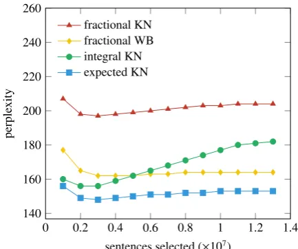
[image:6.595.308.525.64.245.2]. ..fractional KN . ..fractional WB . ..integral KN . ..expected KN
Figure 1: On the language model adaptation task, expected KN outperforms all other methods across all sizes of selected subsets. Integral KN is ap-plied to unweighted instances, while fractional WB, fractional KN and expected KN are applied to weighted instances.
Then we use the weighted subset to train a lan-guage model with expected KN smoothing.
6.2 Experiments
Moore and Lewis (2010) test their method by partitioning the in-domain data into training data and test data, both of which are disjoint from the general-domain data. They use the in-domain training data to select a subset of the general-domain data, build a language model on the se-lected subset, and evaluate its perplexity on the in-domain test data. Here, we follow this experimen-tal framework and compare Moore and Lewis’s unweighted method to our weighted method.
For our experiments, we used all the English data allowed for the BOLT Phase 1 Chinese-English evaluation. We took 60k sentences (1.7M words) of web forum data as in-domain data, further subdividing it into 54k sentences (1.5M words) for training, 3k sentences (100k words) for testing, and 3k sentences (100k words) for fu-ture use. The remaining 12.7M sentences (268M words) we treated as general-domain data.
mini-mize perplexity on thetestset to give it the great-est possible advantage; nevertheless, it is clearly the worst performer. Expected KN consistently gives the best perplexity, and, at the optimal sub-set size, obtains better perplexity (148) than the other methods (156 for integral KN, 162 for frac-tional WB and 197 for fracfrac-tional KN). Finally, we note that integral KN is very sensitive to the subset size, whereas expected KN and the other methods are more robust.
7 Word Alignment
In this section, we show how to apply expected KN to the IBM word alignment models (Brown et al., 1993). This illustrates both how to use expected KN inside EM and how to use it beyond language modeling. Of course, expected KN can be applied to other instances of EM besides word alignment. 7.1 Problem
Given a French sentence f = f1f2· · ·fm and its
English translatione= e1e2· · ·en, an alignmenta
is a sequencea1,a2, . . . ,am, whereai is the index
of the English word which generates the French word fi, or NULL. As is common, we assume that
each French word can only be generated from one English word or from NULL (Brown et al., 1993; Och and Ney, 2003; Vogel et al., 1996).
The IBM models and related models define probability distributionsp(a,f |e, θ), which model how likely a French sentencef is to be generated from an English sentenceewith word alignmenta. Different models parameterize this probability dis-tribution in different ways. For example, Model 1 only models the lexical translation probabilities:
p(a,f |e, θ)∝∏m
j=1
p(fj |eaj).
Models 2–5 and the HMM model introduce addi-tional components to model word order and fer-tility. All, however, have the lexical translation model p(fj | ei) in common. It also contains most
of the model’s parameters and is where overfit-ting occurs most. Thus, here we only apply KN smoothing to the lexical translation probabilities, leaving the other model components for future work.
7.2 Method
Thef andeare observed, whileais a latent vari-able. Normally, in the E step, we collect expected
countsE[c(e,f)] for eacheand f. Then, in the M step, we find the parameter values that maximize their likelihood. However, MLE is prone to over-fitting, one symptom of which is the “garbage col-lection” phenomenon where a rare English word is wrongly aligned to many French words.
To reduce overfitting, we use expected KN smoothing during the M step. That is, during the E step, we calculate the distribution ofc(e,f) for each e and f, and during the M step, we train a language model on bigramse f using expected KN smoothing (that is, withu = e andw = f). This gives a smoothed probability estimate forp(f |e). One question that arises is: what distribution to use as the lower-order distribution p′? Following
common practice in language modeling, we use the unigram distribution p(f) as the lower-order distribution. We could also use the uniform distri-bution over word types, or a distridistri-bution that as-signs zero probability to all known word types. (The latter case is equivalent to a backofflanguage model, where, since all bigrams are known, the lower-order model is never used.) Below, we com-pare the performance of all three choices.
7.3 Alignment experiments
We modified GIZA++ (Och and Ney, 2003) to perform expected KN smoothing as described above. Smoothing is enabled or disabled with a command-line switch, making direct comparisons simple. Our implementation is publicly available as open-source software.1
We carried out experiments on two language pairs: Arabic to English and Czech to English. For Arabic-English, we used 5.4+4.3 million words of parallel text from the NIST 2009 con-strained task,2 and 346 word-aligned sentence
pairs (LDC2006E86) for evaluation. For Czech-English, we used all 2.0+2.2 million words of training data from the WMT 2009 shared task, and 515 word-aligned sentence pairs (Bojar and Prokopov´a, 2006) for evaluation.
For all methods, we used five iterations of IBM Models 1, 2, and HMM, followed by three iter-ations of IBM Models 3 and 4. We applied ex-pected KN smoothing to all iterations of all mod-els. We aligned in both the foreign-to-English
1https://github.com/hznlp/giza-kn
2All data was used except for: United Nations
Alignment F1 Bleu
Smoothing p′ Ara-Eng Cze-Eng Ara-Eng Cze-Eng
none (baseline) – 66.5 67.2 37.0 16.6 variational Bayes uniform 65.7 65.5 36.5 16.6
fractional WB unigramuniform 60.160.8 63.766.5 37.8– 16.9–
zero 60.8 65.2 – –
fractional KN unigram 67.7 70.2 37.2 16.5
expected KN unigramuniform 69.769.4 71.971.3 38.2– 17.0–
[image:8.595.130.467.61.215.2]zero 69.2 71.9 – –
Table 1: Expected KN (interpolating with the unigram distribution) consistently outperforms all other methods. For variational Bayes, we followed Riley and Gildea (2012) in setting αto zero (so that the choice of p′is irrelevant). For fractional KN, we choseDto maximize F1 (see Figure 2).
and English-to-foreign directions and then used the grow-diag-final method to symmetrize them (Koehn et al., 2003), and evaluated the alignments using F-measure against gold word alignments.
As shown in Table 1, for KN smoothing, in-terpolation with the unigram distribution performs the best, while for WB smoothing, interestingly, interpolation with the uniform distribution per-forms the best. The difference can be explained by the way the two smoothing methods estimate p′.
Consider again a training example with a worde
that occurs nowhere else in the training data. In WB smoothing, p′(f) is the empirical unigram
distribution. If f contains a word that is much more frequent than the correct translation of e, then smoothing may actually encourage the model to wrongly align e with the frequent word. This is much less of a problem in KN smoothing, where p′ is estimated from bigram types rather
than bigram tokens.
We also compared with variational Bayes (Ri-ley and Gildea, 2012) and fractional KN. Overall, expected KN performs the best. Variational Bayes is not consistent across different language pairs. While fractional KN does beat the baseline for both language pairs, the value ofD, which we op-timizedDto maximize F1, is not consistent across language pairs: as shown in Figure 2, on Arabic-English, a smaller D is better, while for Czech-English, a largerDis better. By contrast, expected KN uses a closed-form expression forDthat out-performs the best performance of fractional KN.
Table 2 shows that, if we apply expected KN smoothing to only selected stages of training, adding smoothing always brings an improvement,
.
....
0... 0.2 0.4 0.6 0.8 1 64
. 66
. 68
. 70
. 72
.
D .
alignment
F1
.
[image:8.595.310.521.295.473.2]. ..Cze-Eng . ..Ara-Eng
Figure 2: Alignment F1 vs. D of fractional KN smoothing for word alignment.
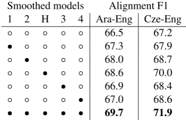
Smoothed models Alignment F1 1 2 H 3 4 Ara-Eng Cze-Eng ◦ ◦ ◦ ◦ ◦ 66.5 67.2 • ◦ ◦ ◦ ◦ 67.3 67.9 ◦ • ◦ ◦ ◦ 68.0 68.7 ◦ ◦ • ◦ ◦ 68.6 70.0 ◦ ◦ ◦ • ◦ 66.9 68.4 ◦ ◦ ◦ ◦ • 67.0 68.6 • • • • • 69.7 71.9
[image:8.595.320.510.550.672.2]with the best setting being to smooth all stages. This shows that expected KN smoothing is consis-tently effective. It is also interesting to note that smoothing is less helpful for the fertility-based Models 3 and 4. Whether this is because modeling fertility makes them less susceptible to “garbage collection,” or the way they approximate the E step makes them less amenable to smoothing, or an-other reason, would require further investigation.
7.4 Translation experiments
Finally, we ran MT experiments to see whether the improved alignments also lead to improved trans-lations. We used the same training data as before. For the Arabic-English tasks, we used the NIST 2008 test set as development data and the NIST 2009 test set as test data; for the Czech-English tasks, we used the WMT 2008 test set as develop-ment data and the WMT 2009 test set as test data. We used the Moses toolkit (Koehn et al., 2007) to build MT systems using various alignments (for expected KN, we used the one interpolated with the unigram distribution, and for fractional WB, we used the one interpolated with the uni-form distribution). We used a trigram language model trained on Gigaword (AFP, AP World-stream, CNA, and Xinhua portions), and minimum error-rate training (Och, 2003) to tune the feature weights.
Table 1 shows that, although the relationship between alignment F1 and Bleuis not very con-sistent, expected KN smoothing achieves the best Bleuamong all these methods and is significantly better than the baseline (p<0.01).
8 Conclusion
For a long time, and as noted by many authors, the usage of KN smoothing has been limited by its restriction to integer counts. In this paper, we ad-dressed this issue by treating fractional counts as distributions over integer counts and generalizing KN smoothing to operate on these distributions. This generalization makes KN smoothing, widely considered to be the best-performing smoothing method, applicable to many new areas. We have demonstrated the effectiveness of our method in two such areas and showed significant improve-ments in both.
Acknowledgements
We thank Qing Dou, Ashish Vaswani, Wilson Yik-Cheung Tam, and the anonymous reviewers for their input to this work. This research was sup-ported in part by DOI IBC grant D12AP00225.
References
Jes´us Andr´es-Ferrer. 2010. Statistical approaches for
natural language modelling and monotone statisti-cal machine translation. Ph.D. thesis, Universidad Polit´ecnica de Valencia.
Amittai Axelrod, Xiaodong He, and Jianfeng Gao. 2011. Domain adaptation via pseudo in-domain data
selection. InProc. EMNLP, pages 355–362.
Maximilian Bisani and Hermann Ney. 2008. Joint-sequence models for grapheme-to-phoneme
conver-sion.Speech Communication, 50(5):434–451.
Ondrˇej Bojar and Magdalena Prokopov´a. 2006.
Czech-English word alignment. In Proc. LREC,
pages 1236–1239.
Peter F. Brown, Stephen A. Della Pietra, Vincent J. Della Pietra, and Robert L. Mercer. 1993. The mathematics of statistical machine translation:
Pa-rameter estimation. Computational Linguistics,
19:263–311.
Stanley F. Chen and Joshua Goodman. 1999. An empirical study of smoothing techniques for
lan-guage modeling. Computer Speech and Language,
13:359–394.
A. P. Dempster, N. M. Laird, and D. B. Rubin. 1977. Maximum likelihood from incomplete data via the
EM algorithm. Journal of the Royal Statistical
So-ciety, Series B, 39:1–38.
Jianfeng Gao, Joshua Goodman, Mingjing Li, and Kai-Fu Lee. 2002. Toward a unified approach to
statisti-cal language modeling for Chinese. ACM
Transac-tions on Asian Language Information, 1:3–33.
Joshua T. Goodman. 2001. A bit of progress in lan-guage modeling: Extended version. Technical Re-port MSR-TR-2001-72, Microsoft Research.
Joshua Goodman. 2004. Exponential priors for
maxi-mum entropy models. InProc. HLT-NAACL, pages
305–312.
Yili Hong. 2013. On computing the distribution
func-tion for the Poisson binomial distribufunc-tion.
Compu-tational Statistics and Data Analysis, 59:41–51.
Dietrich Klakow. 2000. Selecting articles from the
language model training corpus. InProc. ICASSP,
Reinhard Kneser and Hermann Ney. 1995. Improved
backing-off for M-gram language modeling. In
Proc. ICASSP 1995, pages 181–184.
Philipp Koehn, Franz Josef Och, and Daniel Marcu.
2003. Statistical phrase-based translation. InProc.
HLT-NAACL, pages 127–133.
Philipp Koehn, Hieu Hoang, Alexandra Birch, Chris Callison-Burch, Marcello Federico, Nicola Bertoldi, Brooke Cowan, Wade Shen, Christine Moran, Richard Zens, Chris Dyer, Ondrej Bojar, Alexandra Constantin, and Evan Herbst. 2007. Moses: Open source toolkit for statistical machine translation. In
Proc. ACL, Companion Volume, pages 177–180. Sung-Chien Lin, Chi-Lung Tsai, Lee-Feng Chien,
Keh-Jiann Chen, and Lin-Shan Lee. 1997. Chinese lan-guage model adaptation based on document classifi-cation and multiple domain-specific language
mod-els. InProc. Eurospeech, pages 1463–1466.
Robert Moore and William Lewis. 2010. Intelligent
selection of language model training data. InProc.
ACL, pages 220–224.
Hermann Ney, Ute Essen, and Reinhard Kneser. 1994. On structuring probabilistic dependencies in
stochastic language modelling. Computer Speech
and Language, 8:1–38, 1.
Franz Josef Och and Hermann Ney. 2003. A sys-tematic comparison of various statistical alignment
models. Computational Linguistics, 29(1):19–51.
Franz Josef Och. 2003. Minimum error rate training in
statistical machine translation. InProc. ACL, pages
160–167.
Darcey Riley and Daniel Gildea. 2012. Improving the IBM alignment models using variational Bayes. InProc. ACL (Volume 2: Short Papers), pages 306– 310.
Andreas Stolcke. 2002. SRILM – an extensible
lan-guage modeling toolkit. InProc. International
Con-ference on Spoken Language Processing, volume 2, pages 901–904.
Martin Sundermeyer, Ralf Schl¨uter, and Hermann Ney. 2011. On the estimation of discount parameters for
language model smoothing. In Proc. Interspeech,
pages 1433–1436.
Yik-Cheung Tam and Tanja Schultz. 2008. Correlated bigram LSA for unsupervised language model
adap-tation. InProc. NIPS, pages 1633–1640.
Yee Whye Teh. 2006. A hierarchical Bayesian lan-guage model based on Pitman-Yor processes. In
Proc. COLING-ACL, pages 985–992.
Stephan Vogel, Hermann Ney, and Christoph Tillmann. 1996. HMM-based word alignment in statistical
translation. InProc. COLING, pages 836–841.
Joern Wuebker, Mei-Yuh Hwang, and Chris Quirk. 2012. Leave-one-out phrase model training for
large-scale deployment. InProc. WMT, pages 460–