Munich Personal RePEc Archive
The Effects of Temporal Aggregation on
Search Engine Data
Tierney, Heather L.R. and Kim, Jiyoon (June) and Nazarov,
Zafar
Indiana University-Purdue University Fort Wayne, Indiana
University-Purdue University Fort Wayne, Indiana
University-Purdue University Fort Wayne
30 January 2018
Online at
https://mpra.ub.uni-muenchen.de/84474/
The Effects of Temporal Aggregation
on Search Engine Data
By
Heather L.R. Tierney,
Jiyoon Kim, and Zafar Nazarov
Abstract
Using structured machine learning, this paper examines the effect that temporal aggregation has on big data from Google Analytics and Google Trends. Specifically, daily and weekly data from the Charleston Area Convention and Visitors Bureau (CACVB) website from January 2008 to March 2009 via Google Analytics and weekly, monthly, and quarterly data from Google Trends for seven economic variables from 2004 to 2011 are examined. Taking into account the different levels of aggregation, the CDFs and the estimated regression results are examined. The Kolmogorov-Smirnov test rejects the null of equivalent data distributions in the vast majority of cases for the CACVB data, but this is not the case for the economic variable. Through data mining, this paper also finds that aggregation has the potential of affecting the level of integration and the regression results for both the CACVB data and the seven economic variables.
KEYWORDS: Big Data, Machine Learning, Data Mining, Aggregation, Unit roots,
Scaling Effects, Normalization Effects
JEL Classification Codes: C55, C43, C19
1.
Introduction
Search engine data is one form of big data and it is a new source for time
series data, which is able to capture economic and societal trends almost
instantaneously. This has led to the relatively new field of nowcasting in economics,
finance, and business. Big data lends itself exceedingly well to machine learning and
data mining, which refers to the ability to obtain new information from the existing
data (Jun, Yoo, and Choi 2017; Fürnkranz, Gamberger, and Lavrač 2012).
Nowcasting refers to using the past to predict the present or the very near future
and structured machine learning techniques permit us to find these trends.
One type of big data used in this paper is from Google Trends, which provides
an index of the volume of web searches for a specific key word or phrase such as
‘mortgage defaults’ in the U.S.1 Graph 3A demonstrates that pre-2005, the search for
‘mortgage defaults’ is virtually non-existent, but gradually, interest begins to builds
in March 2007 until it hits a peak in September 2008, which is consistent with the
start of the Financial Crisis of 2008. A similar story unfolds in Graph 3B regarding
‘gold price,’ which hits its peak in March 2008 since investors turn to gold during times of economic turmoil.
With this new source of data generating a great deal of research especially in
machine learning area, it is important to understand the properties of this data
given that his data has been previously normalized and scaled. Specifically, this
paper studies the effect of aggregation on Google Analytics, another source of big
data, and Google Trends data by examining the cumulative distribution functions
(CDFs) and the estimated regression output, which are important for forecasting
and policy-making decisions.
If the data characteristics are being distorted with higher levels of
aggregation, then this could cause a loss of information. Many of the economic
models use either monthly or quarterly data and, often, the data is transformed in
1 Google Trends was formerly known as Google Insights. The web address for Google Insights is:
http://www.google.com/insights/search/, which now take you to the same website for Google Trends, http://www.google.com/trends. Additional sources of search engine data can be obtained from Google Analytics, http://www.google.com/analytics/ (Horák, Ivan, Kukuliač, Inspektor,
order to obtain the desired level of aggregation, which is why it is crucial to better
understand the effects of aggregation on regressions results.
Previous work relating to aggregation and the use of normalized and scaled
variables posed some problematic findings.2 For instance, in the field of information
technology (IT), as it relates to the central processing unit, memory, bandwidth
usage, etc., Marvasti (2010) has found that aggregation affects the data distribution
and decreases the data range, which affects the tail regions. Analogously, when
using search engine data, Tierney and Pan (2013) find that the level of dispersion
generally changes from under- to over-dispersion when using daily and weekly data
to examine the relationship between website traffic and search volume data.
Along the lines of Marvasti (2010), this paper examines the effect of temporal
aggregation on the CDFs of time series data obtained from Google Trends and
Google Analytics through the use of the two-sample Kolmogorov-Smirnov (KS) test.
Regarding the estimated regression results, the averaging or aggregation of
data has the potential of adversely affecting the estimated parameters of the model
and the RSS, which specifically affects the variance and the estimated test statistics
(Granger and Siklos 1995, Rossana and Seater 1995, Marcellino (1999), Garrett
2002).
According to Garrett (2002), the aggregated coefficient is supposed to be the
sum of the coefficients from the regression using the less aggregated data. This
paper does not find this to be the case when using data from either Google Analytics
or Google Trends.
In order to study the effects of temporal aggregation on search engine data,
this paper uses data from two sources. The first source of data is daily and weekly
data for six search volume time series that are obtained from the Charleston Area
Convention and Visitors Bureau (CACVB) website from January 2008 to March 2009
which is obtained using Google Analytics.3 The second source of data involves
weekly data from Google Trends for seven variables of potential economic interest,
2Aggregation has the potential to add ‘noise’ while making it harder to separate the trend, i.e. long
-run fluctuations from the cycle, which refers to short--run fluctuations (Garrett 2002).
which from now on will be referred to as the economic dataset. These variables are
‘unemployment,’ ‘inflation,’ ‘mortgage defaults,’ ‘US deficits,’ ‘GDP,’ ‘economic growth,’
and‘gold price.’
The CDFs of the daily and weekly data of the CACVB website are tested using
the two-sample KS test evaluated at the 5% significance level in order to determine
if they are statistically equivalent. Regarding the economic dataset, the weekly data
is transformed into monthly and quarterly data. The KS test is used to compare the
CDFs of the weekly data against the aggregated versions of monthly and quarterly
data.
The structure of this paper is as follows: Section 2 presents a brief discussion
of the data; Section 3 presents the methodology; and Section 4 contains the
empirical results and Section 5 conclusion.
2.
Discussion of the Data
Google Trends does not provide the raw big data; it readily provides weekly
data, and it can provide daily and weekly data that requires a specialized program in
order to obtain the daily search volume results, which is how the CACVB data has
been obtained. Both the daily and weekly data have been normalized and then
scaled. Each data point reflects the ratio of the number of searches for a particular
key word or phrase to the total number of searches done on using the Google search
engine during a given week (Google Trends 2011c).
The normalization process refers to dividing the dataset by a particular
variable in order to remove the variable’s effect of the data so that the absolute
rankings may be obtained. This is to remove the effect of geographic areas with the
largest search volumes from always being ranked higher. The problem when it
comes to interpreting the data is that the same index number for two different
regions does not reflect the same search volume levels but how likely they are to
search for a particular key word or phrase (Google Trends 2011a). The scaling
process reduces the range of the data to be between 0 and 100 with each data point
The CDFs obtained from five quarters of daily data are tested against the
CDFs of the weekly data of the CACVB website, which are obtained from Google
Anayltics. Four of the CACVB search volume variables are obtained from a universal
search in all categories and are denoted by (all), which follows the variable. The
remaining two of the CACVB search volume variables are restricted to searchs only
within the travel category and are followed by the term (travel). The variables are
as follows: ‘charleston sc’ (all), ‘charleston hotels’ (all), ‘charleston restaurants’ (all),
‘charleston travel’ (all), ‘charleston sc’ (travel), and‘charleston hotels’ (travel). Table
1A provides a summary of the variables along with their abbreviations, Table 2A
provides the number of observations, and Table 3A provides their exact data
samples, which ranges from January 2008 to March 2009.
To construct the CDFs, the level data is used while the log forms of the data
are used for the structured machine learning, which pertains to the regressions with
the intent of data mining, i.e. obtaining new information using big data
(Fürnkranz, Gamberger, and Lavrač 2012). The log forms of the data aids in the
interpretation of the estimated regression coefficients and it helps to reduce the
magnitude of the regressand, which is "Y_all_visits" (all) for the regressions
involving the CACVB data. "Y_all_visits" (all) is all the website traffic, i.e. the number
of hits to the CACVB website during the given time period and its frequency is in
both the daily and weekly versions.
The regressand "Y_all_visits" (all) is data that has not been normalized and
scale, and so it is possible to see the magnitude of big data with respect to just the
CACVB website. The mean for the weekly version of "Y_all_visits" (all) is 24,808.90
hits with the minimum being 13,893 and the maximum being 32,773 hits from
January 2008 to March 2009.
Search engine data is count data but it is also time series data, which means
there could be stationarity issues.4 It is important to test for unit roots because it
impacts the test statistics from the structured machine learning results. To test for
stationarity, the Augmented Dickey-Fuller (ADF) and the Elliott-Rothenberg-Stock
4 Hellström (2002), Pavlicek, J. and Kristoufek, L. (2015), and Kristoufek, Moat, and Preis (2016)
Point Optimal Test, which is now referred to as ERS, are used (Said and Dickey1984,
Elliot, Rothenberg, and Stock 1996).
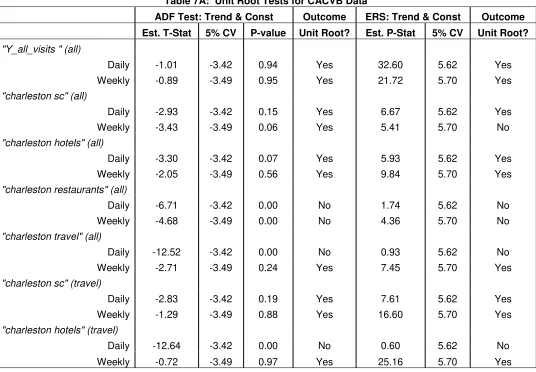
One interesting finding of this paper is that the level of stationarity can differ
with the level of aggregation. A summary of the unit root results with the inclusion
of a constant term and a time trend for the CACVB data can be found in Table 7A.5 A
unit root is found in both the daily and weekly data of "Y_all_visits" (all), charleston
hotels’ (all), and ‘charleston sc’ (travel). The daily and weekly data of ‘charleston
restaurants’ (all) are found to be stationary.
Both the ADF and ERS tests find the daily data of ‘charleston travel’ (all) and
‘charleston hotels’ (travel) to be stationary while the weekly version to contain a unit root. When the level of integration differs with the level of aggregation, this makes
comparing the regression output much more difficult.
Unit root tests are known to have low power, so it is understandable that
there would be some conflicting results.6 The ADF and ERS test obtain conflicting
results with respect to the weekly data of ‘charleston sc’ (all). The ADF test finds a unit root while the ERS test does not.
The ADF and ERS tests finds the regressand, the log of "Y_all_visits" (all) to
contain a unit root for both the daily and weekly data. Hence, the first difference of
the log of "Y_all_visits" (all) is used in all the estimated regressions involving the
CACVB data.
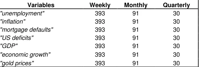
Table 1B presents a list of the search volume variables examined, which are
‘unemployment,’ ‘inflation,’ ‘mortgage defaults,’ ‘US deficits,’ ‘GDP,’ ‘economic growth,’
and‘gold price’ with Table 2B presenting the number of observations for the weekly, monthly, and quarterly data. The data range for the economic dataset is from 2004
to 2011 with more detail being presented in Table 3B.
For the regressions, the log versions of ‘unemployment,’ ‘inflation,’ ‘GDP,’
‘economic growth,’ and‘gold price’ are used since ‘mortgage defaults’ and ‘US deficits’
5 Sequential testing of the data using the ADF and ERS tests have been applied to the data and the
aforementioned results hold.
6 Having low power refers to the occurrence of a Type II error, which is failing to reject the null when
have too many missing observations. The unit root testing of the economic dataset
proved to be more conflicted as is shown in Table 7B.
The ADF and ERS tests find unit roots in the weekly and monthly versions of
‘unemployment’ but they differ with respect to quarterly data. The ADF finds a unit root while the ERS test does not. The weekly and monthly versions of ‘inflation,’ are stationary. The ADF test using quarterly data of ‘inflation’ finds stationarity while the ERS test finds a unit root. There appears to be stationarity in the weekly and
monthly data of ‘GDP’ anda unit root in the quarterly data of ‘GDP’ according to both the ADF and ERS tests.
The ADF and ERS tests are in disagreement regarding ‘economic growth’ except for the weekly data version where they find stationarity. For the monthly
version of ‘economic growth,’ the ADF test finds it to be stationary and the quarterly version to be non-stationary and the ERS test obtains the opposite results.
For ‘gold price,’ the ADF and ERS tests find the weekly version to be stationary and the quarterly version to be non-stationary. There is dissent with
respect to the monthly version of ‘gold price.’ The ADF finds the monthly version to be stationary while the ERS test finds a unit root.
3.
The Methodology
3.1 Examining the CDFs
The reason for utilizing the two-sample KS test over some other empirical
density test is that it permits the comparison of two empirical CDFs.7 For this
paper, the CDFs of the aggregated data is compared to a benchmark CDF in the
two-sample KS test, which is a nonparametric test for comparing two empirical
distributions (Kim 1969, Kim and Jennrich 1973, Marvasti 2010). In this case the
term, nonparametric refers to comparing two empirical CDFs of the variables, X and
Y with the total number of observations being M and N respectively. The empirical
CDFs for X and Y are as follow:
1
1 M
X m
m
F x P X x I X x
M
(1)
7 The other empirical density tests are designed to compare one empirical CDF against an alternate
and
1 1 N Y N nF y P Y y I Y y
N
(2)The benefits of using the KS test are that it is robust, not sensitive to scaling,
and works well when the data is not from the normal distribution. The KS test is
problematic when the data is normal. Hence, it is important to test for the normality
of the data, which is done using the following normality tests: Lilliefors, Cramer-von
Mises, Anderson-Darling, and Watson empirical distribution tests and the
Jarque-Bera Normality Test (Stephens 1970, Stephens 1974). The null hypothesis for the
aforementioned tests is that the data is normal.
There are various forms of the KS test, especially as it pertains to obtaining
the critical values (CV), so it is important to discuss the specific form used, which is
the one specified by Capon (1965). Regarding the KS test, the hypothesis test
concerns the CDFs of X and Y and is of the following form: H F0: X FY versus
1: X Y
H F F . FX and FYwill differ by some amount , and so the KS test amounts to measuring the distance, DXbetween theFX and FYthat is greater than , i.e.
sup
X X Y x
D F x F x
(3)
The KS test statistic, KSX is as follows:
1 2
sup
X X Y
x
mn
KS F x F x
m n
(4)
If the null hypothesis fails, then
1 1
2 2
X X
mn mn
KS D
m n m n
(5)
which means that a threshold gneeds to be determined based on the CV that is 5%
for this paper. The CV depends upon the threshold g and the KS distribution
H and is as follows:
1 2
0 0 X 0 1
mn
P H H P KS g H H g
m n
Hence, the KS test amounts to testing:
1 2
0: X * CV of the KS distribution
mn
H KS g
m n
1 2
1: X * CV of the KS distribution
mn
H KS g
m n
with the CV values for the large sample approximation obtained from Massey
(1951) and the tables of Miller (1956). For this paper, the CV for the CACVB data is
1.33 using the tables provided by Miller (1956) and is 1.33 for the KS test involving
monthly data and 1.32 when using quarterly data for the economic dataset. The
large sample CV approximation is 1.36 for both datasets.
3.2 Examining the Estimated Structured Machine Learning Results
The type of machine learning used in this paper is structured machine
learning in the form of regression analysis (Alpaydin 2009; Fürnkranz, Gamberger,
and Lavrač 2012). The purpose of these regressions is to compare the effect of
aggregation on the estimate regression coefficients and the RSS. According Garrett
(2002), estimated regression results demonstrate a certain pattern. The sum of the
estimate coefficients from the less aggregated data should sum to the estimate
coefficient of the aggregated data. For the CACVB dataset, the regressand is the log
of "Y_all_visits" (all) and the regressors being the log verisons of ‘charleston sc’ (all),
‘charleston hotels’ (all), ‘charleston restaurants’ (all), ‘charleston travel’ (all),
‘charleston sc’ (travel), and ‘charleston hotels’ (travel) with each being run as a
separate regression.
For example, for the daily CACVB data, the first difference of the log of
"Y_all_visits" (all) is regressed onto the log of ‘charleston sc’ (all) and six lags to
account for the 7-day week. With the exclusion of the constant term, the seven
estimated regression coefficients are summed and then compared to the estimated
coefficients of the weekly data with the regressand also being the first difference of
the log of "Y_all_visits" (all). This is done for the remaining regressors taking into
Regarding the economic dataset, an AR(p) model is used with the p-lags
depending on the level of aggregation. The weekly data is compared to the monthly
data and the monthly data is compared to the quarterly data. Hence, the regressions
with the weekly data have 4 lags, which are then compared to their monthly
counterparts, which have only 1 lag. Alternatively, when comparing the monthly
data to the quarterly data, the regressions with the monthly data have 3 lags while
the regressions with the quarterly data have only 1 lag.
4.
Empirical Results
4.1 Empirical Results of the CDFs
Since access to the raw data is not permitted due to Google’s privacy policy,
each of the CDFs of the daily data is measured against the weekly data in the CACVB
dataset (Barbaro and Zeller 2006). Analogously, in the economic dataset, the
weekly dataset is used at the benchmark against the monthly and quarterly data.
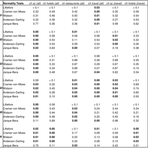
The results for the tests for normality of Lilliefors, Cramer-von Mises,
Anderson-Darling, and Watson empirical distribution tests and the Jarque-Bera
Normality Test are presented in Table 5A for the CACVB data and in Table 5B for the
economic data. The p-values in bold print in Tables 5A and 5B indicate that the null
of normality is rejected at the 5% significance level. Due to the low power of the
normality tests, there are some contradictory findings. All the normality tests reject
normality for the variable ‘charleston sc’ (all) in the second, third, fourth, and fifth
quarters except for the Lilliefors test in the fourth quarter and the Jarque-Bera test
in the fifth quarter when using daily data. When using weekly data, the null of
normality is rejected for all the normality tests except for the Jarque-Bera test with
respect to the variable ‘charleston sc’ (all). For the variable ‘charleston restaurants’
(all), the null of normality fails to be rejected for most of the hypothesis tests when
using daily data in the first, second, and third quarters as well as in the weekly data.
The Lilliefors test rejects the null of normality in the second quarter of daily data for
the second quarter of daily data and for the weekly data as well. The majority of the
normality tests for the remaining quarters using daily data fails to reject normality.
The CDFs of the six search volume variables using the daily data from the
fourth quarter and the weekly data of the CACVB website demonstrates that there is
a noticeable gap between both CDFs, which is shown in Graphs 1A through 1F. The
ranges of the CACVB data is given in Table 4A. The range for the search volume
index of ‘charleston hotels’ (all) for weekly data is from 3 to 7 and the range for the daily data is from 26 to 100, which accounts for the CDFs in Graph 1B.
Table 6A provides the KS test results with the statistically significant results
in bold print. With only three exceptions of the first quarter of ‘charleston sc’ (all)
and the first and third quarter of ‘charleston sc’ (travel), the null of statistically equivalent CDFs is rejected even when using the more conservative CV of 1.36 as is
provided by Massey (1951).
Concerning the economic dataset, the null of normality fails to be rejected for
the vast majority of variables as is demonstrated in Table 5B for the monthly and
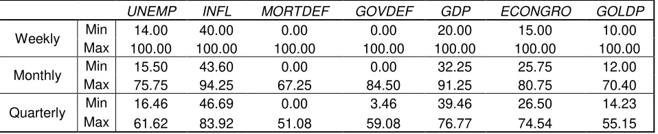
quarterly aggregated search volume variables. The ranges of the variables of the
economic dataset are presented in Table 4B and as Marvasti (2010) noted, the
ranges decrease with higher levels of aggregation.
The null of normality is rejected at the 5% significance level for weekly,
monthly, and quarterly ‘unemployment’ data except for the Jarque-Bera test when using quarterly data. Weekly ‘mortgage defaults,’ ‘US deficits,’ ‘GDP,’ ‘economic
growth,’ and‘gold price,’ all reject the null of normality at the 5% significance level, which is not necessarily the case when using monthly and quarterly data. ‘inflation’ fails to reject the null of normality except for the Lilliefors test when using weekly
data. Hence, there are conflicting results with respect to the normality tests and the
various levels of aggregation concerning the economic dataset.
The CDF graphs of the weekly and quarterly data for the economic dataset
are presented in Graphs 2A through 2G, and as one can see that there is very little
difference between the two CDFs. The graph with the largest difference between
less than the CV of 1.36, the null of equivalent empirical CDFs fails to be rejected. In
fact, the null of equivalent empirical CDFs fails to be rejected for the two-sample KS
test involving either monthly or quarterly data.
4.2 Estimated Structured Machine Learning Results
Just as with the comparison of the CDFs, when using the CACVB dataset, the
estimated structured machine learning results also find there to be no agreement
between the daily and weekly data, which are given in Tables 8 and 9. Tables 8 and
9 provide the regressions results for the first difference and the level version of the
log of the regressors when there is disagreement between the ADF and ERS tests or
disagreement with the level of integration based on the aggregation level.
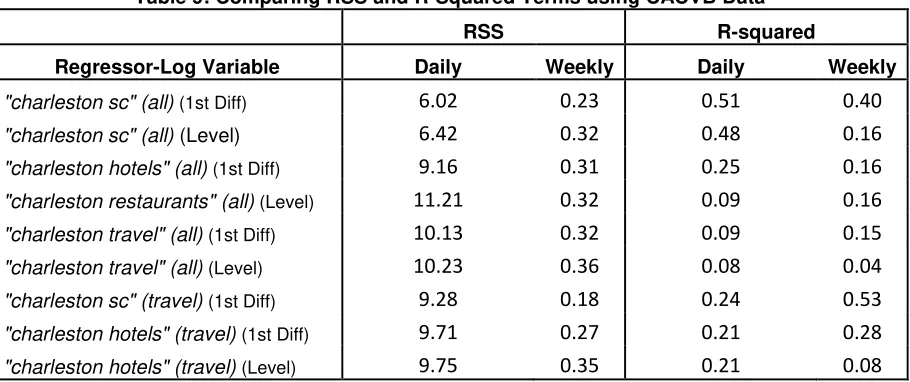
As indicated by Garrett (2002), the RSS of the regressions in the less
aggregated data, i.e. the daily data are greater than the RSS of the regressions using
the weekly data as is demonstrated in Table 9. So, it is not surprising that most of
the estimated coefficients of the regressions using the weekly data are statistically
significant with the exception of ‘charleston travel’ (all) since the RSS are smaller. The sum of the estimated regression coefficients when using the daily data
also differs from its weekly data counterpart. For instance, the sum of the daily
coefficients of all the regressors are negative with the exception of "charleston
travel" (all) and the estimated coefficient from the regression with the weekly data
are all positive.
As has been previously stated, the monthly and quarterly versions of the data
in the economic dataset are formed from weekly data. Aggregating data before
performing a regression is commonplace in most fields such as economics, finance,
and business. This paper analyzes the effect of aggregating the data before
performing a regression.
Furthermore, comparing regressions results from data with different levels
of aggregation and different levels of integration is proving to be problematic
especially with respect to the economic dataset. In terms of statistical significance,
the regressions using the weekly data fare better than the regressions using the
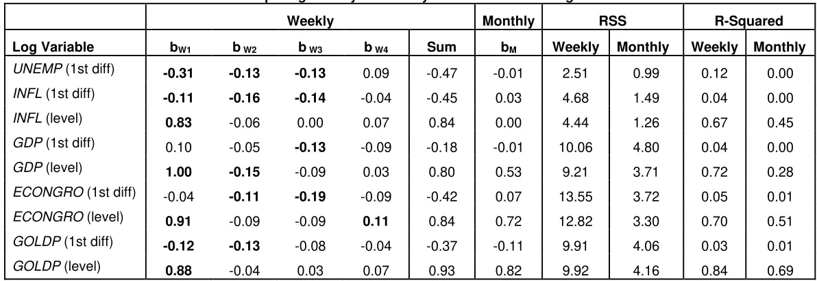
The regression results for the economic dataset are provided in Tables 10
and 11. The estimated coefficient of the first lag in the regression using monthly
data are statistically insignificant except for the regression involving the level form
of inflation, where the estimated coefficient is 0.0001. In this instance, the opposite
of what Garrett (2002) expects is obtained. The sum of the estimate coefficients
using the weekly data do not match their monthly counterpart. The RSS of the
regressions using monthly data are smaller than the regressions using weekly data.
It should be noted that the R-squared terms for the regressions using
monthly data is 0.00 or 0.01 for the first difference of the log of ‘unemployment,’
‘inflation,’ ‘GDP,’ ‘economic growth,’ and ‘gold price.’ Actually, this is not surprising because the monthly versions of ‘inflation’ and‘GDP’ are stationary and the ADF and ERS tests are conflicted when it comes to monthly ‘economic growth,’ and ‘gold
price.’
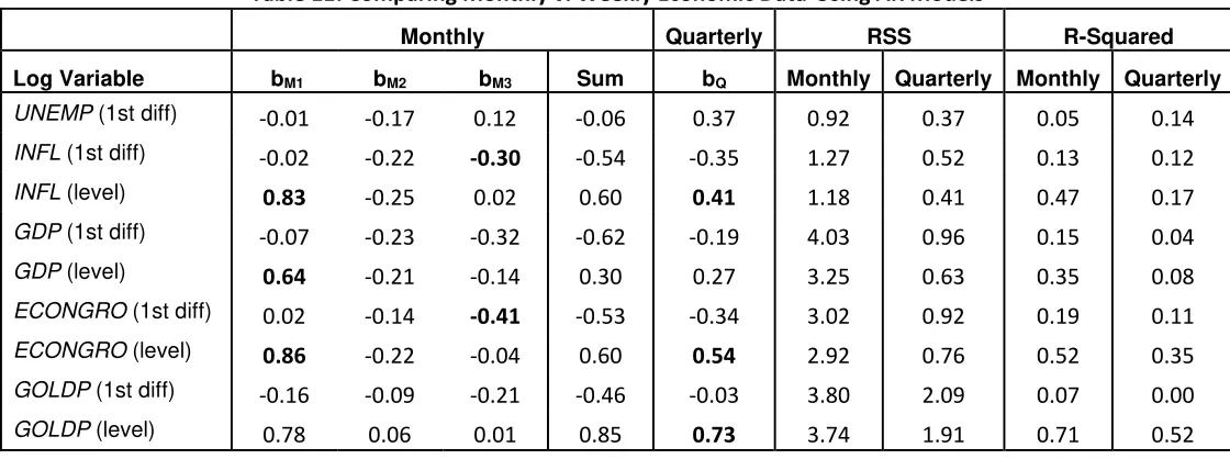
Regarding the comparison of the estimated regressions coefficients of
monthly and weekly data, the only statistically significant coefficients are the level
form of the log versions of ‘inflation,’ ‘economic growth,’ and ‘gold price.’ The ADF and ERS tests produce contrary results for the quarterly versions of ‘inflation’ and
‘economic growth,’but quarterly ‘gold price’ is considered to be stationary. It should be noted that the regression using the first difference of the log of ‘gold price’ has an R-squared value of 0.00, meaning that the model is not captured by an AR(1), which
makes it difficult to compare estimated regression results.
As is the case with the CACVB dataset, the sum of the estimated coefficients
of the regressions revolving monthly data are not equivalent of their quarterly
counterpart as is shown in Table 11.
Hence, when it comes to estimating regressions, caution needs to be used in
aggregating the data and more importantly, in interpreting the data. For example,
estimated regression results obtained from less aggregated data should not be used
5.
Conclusion
This paper looks at two sources of big data with the intent of examining
whether or not temporal aggregation affects the CDFs and the estimated structured
machine learning results. Specifically, two different types of data are examined: the
CACVB dataset, which uses data from Google Analytics, and the economic dataset,
which uses data from Google Trends.
The CACVB data provides daily and weekly data that already have been
normalized and scaled. Regarding the economic dataset, the monthly and quarterly
versions of the economic dataset are aggregated from the normalized and scaled
weekly data, which is a regularly used method of aggregation in the field of
economics.
Regarding the CDFs of the CACVB data and the economic dataset, the KS test
rejects the null of equivalent data distributions in the vast majority of cases for the
CACVB data using daily and weekly data with only three exceptions, which are the
first quarter of ‘charleston sc’ (all) and the first and third quarter of ‘charleston sc’
(travel).
The findings in the economic dataset are opposite of that of the CACVB
dataset with respect to the CDFs. For the economic data set, the CDFs of the weekly
data is compared to the CDFs of the monthly and quarterly data. Based upon the
two-sample KS test, it appears that aggregating the data after it has been normalized
and scaled does not affect the data distribution but it does decrease the range as
evidenced by the results regarding the economic dataset.
Regarding the structured machine learning portion of this paper, it is
important to test for the unit roots with each level of aggregation. It is possible for
less aggregated data to be stationary while higher levels of aggregation can be
non-stationary, which occurs in both the CACVB and the economic datasets.
In addition, when both the CACVB dataset and the economic data set are used
in regressions, which is the form of structured machine learning used in this paper,
it appears that aggregation affects the estimated coefficients. The sum of the
estimated coefficients of the regressions using weekly data. For the economic
dataset, the same pattern of the sum of the estimated coefficients of the regressions
using less aggregated data do not come close to the estimated coefficients of the
regressions using more aggregated data.
In conclusion, when using big data from Google Analytics and Google Trends,
it is important to take note of the structure of the data for data mining purposes.
Inferences pertaining to less aggregated data cannot be extrapolated to higher levels
of aggregation as has been demonstrated using both the CACVB and the economic
References
Alpaydin, E. (2009), Introduction to Machine Learning, 2nd Ed, The MIT Press,
Cambridge, Massachusetts.
Azar, J. (2009), “Oil Prices and Electric Cars”, Princeton University Working Paper.
Barbaro, M. and Zeller, T. (2006), “A Face Is Exposed for AOL Searcher No.
4417749”, New York Times, August 9, accessed online at http://www.nytimes.com.
Capon, J. (1965), “On the Asymptotic Efficiency of the Kolmogorov-Smirnov,” Journal
of the American Statistical Association, 60:311, 843-853.
Elliot, G., Rothenberg, T.J. and Stock, J.H. (1996). “Efficient Tests for an
Autoregressive Unit Root,” Econometrica, 64, 813-836.
Fürnkranz, J., Gamberger, D., Lavrač, N. (2012), Foundations of Rule Learning, Springer-Verlag, Berlin Heidelberg.
---Google Trends (2011a), “How is the data normalized?”
http://www.google.com/support/insights//bin/bin/answer.py?answer=87284 (accessed July 7, 2011).
---Google Trends (2011b), “How is the data scaled?”
http://www.google.com/support/insights//bin/bin/answer.py?answer=87282 (accessed July 7, 2011).
---Google Trends (2011c), “What do the numbers on the graph mean?”
http://www.google.com/support/insights/bin/answer.py?hl=en&answer=87285 (accessed July 7, 2011).
Granger, C. W. J., and Siklos, P.L. (1995), ‘‘Systematic Sampling, Temporal Aggregation, Seasonal Adjustment, and Cointegration: Theory and Evidence.’’
Journal of Econometrics, 66:2, 357–369.
Hellström, J. (2002), Count Data Modelling and Tourism Demand. Umeå Economic
Studies N.584.
Horák J., Ivan I., Kukuliač P., Inspektor T., Devečka B., Návratová M. (2013), “Google
Jun, S.-P., Yoo, H.S., and Choi, S. (2017), “Ten Years of Research Change using Google Trends: From the Perspective of Big Data Utilizations and Applications.” Technological Forecasting & Social Change,
https://doi.org/10.1016/j.techfore.2017.11.009
Kim, P.J. (1969), “On the Exact and Approximate Sampling Distribution of the Two
Sample Kolmogorov-Smirnov Criterion Dm n, ,m n ,” Journal of the American
Statistical Association, 64: 328, 1625-1637.
Kristoufek, L., Moat, H.S., and Preis, P. (2016), “Estimating Suicide Occurrence
Statistics Using Google Trends,” European Physical Journal (EPJ) Data Science,” 5:32.
DOI 10.1140/epjds/s13688-016-0094-0
Kim, P.J. and Jennrich, R.I. (1973), "Tables of the Exact Sampling Distribution of the Two-sample Kolmogorov-Smirnov Criterion Dm n, ,m n ," Selected Tables in
Mathematical Statistics: Vol I, H.L. Harter and D.B. Owen, eds., Chicago: Markham
Publishing Co, 79-170.
Marvasti, M.A. (2010), “Quantifying Information Loss through Data Aggregation,”
VMware Technical White Paper, 1-14.
Marcellino, M. (1999), ‘‘Some Consequences of Temporal Aggregation in Empirical
Analysis.’’Journal of Business and Economic Statistics, 17:1, 129–136.
Massey, F.J. (1951), "The Kolmogorov-Smirnov Test for Goodness of Fit," Journal of
the American Statistical Association, 46:253, 68-77.
Miller, L.H. (1956), “Table of Percentage Points of Kolmogorov Statistics,” Journal of
the American Statistical Association, 51:273, 111-121.
Pavlicek, J. and Kristoufek, L. (2015), “Nowcasting Unemployment Rates with Google Searches: Evidence from the Visegrad Group Countries,”PLoS ONE, 10(5), e0127084. http://doi.org/10.1371/journal.pone.0127084
Rossana, R. J., and Seater, J.J. (1995), ‘‘Temporal Aggregation and Economic Time Series,’’ Journal of Business and Economic Statistics, 13:4, 441–451.
Said, S. E., and Dickey, D. A. (1984), “Testing for Unit Roots in Autoregressive-Moving Average Models of Unknown Order.” Biometrika 71, 599–607.
Stephens, M. A. (1970), “Use of the Kolmogorov-Smirnov, Cramer-Von Mises and Related Statistics Without Extensive Tables,” Journal of the Royal Statistical Society.
Stephens, M. A. (1974), “EDF Statistics for Goodness of Fit and Some Comparisons,”
Journal of the American Statistical Association, 69:347, 730-737.
Tierney, H. L. R. and Pan, B. (2013), “A Poisson Regression Examination of the
Relationship between Website Traffic and Search Engine Queries,” NETNOMICS:
0.0 0.2 0.4 0.6 0.8 1.0
40 50 60 70 80 90 100
Daily Data: Quarter 4 Weekly Data P ro b a b il it y Graph 1A CDFs of "charleston sc" (all)
0.0 0.2 0.4 0.6 0.8 1.0
10 20 30 40 50 60 70 80 90 100 Daily Data: Quarter 4
Weekly Data P ro b a b il it y Graph 1B CDFs of "charleston hotels" (all)
0.0 0.2 0.4 0.6 0.8 1.0
30 40 50 60 70 80 90 100
Daily Data: Quarter 4 Weekly Data P ro b a b il it y Graph 1C CDFs of "charleston restaurants" (all)
0.0 0.2 0.4 0.6 0.8 1.0
0 10 20 30 40 50 60 70 80 90 100
Daily Data: Quarter 4 Weekly Data P ro b a b il it y Graph 1D CDFs of "charleston travel" (all)
0.0 0.2 0.4 0.6 0.8 1.0
30 40 50 60 70 80 90 100
Daily Data: Quarter 4 Weekly Data P ro b a b il it y Graph 1E CDFs of "charleston sc" (travel)
0.0 0.2 0.4 0.6 0.8 1.0
20 30 40 50 60 70 80 90 100
0.0 0.2 0.4 0.6 0.8 1.0
20 30 40 50 60 70 80 90 100
Weekly Data Quarterly Data
P ro b a b il it y Graph 2A CDFs of "economic growth"
0.0 0.2 0.4 0.6 0.8 1.0
20 30 40 50 60 70 80 90 100
Weekly Data Quarterly Data
P ro b a b il it y Graph 2B CDFs of "GDP"
0.0 0.2 0.4 0.6 0.8 1.0
10 20 30 40 50 60 70 80 90 100
Weekly Data Quarterly Data
P ro b a b il it y Graph 2C CDFs of "gold prices"
0.0 0.2 0.4 0.6 0.8 1.0
0 10 20 30 40 50 60 70 80 90 100
Weekly Data Quarterly Data
P ro b a b il it y Graph 2D CDFs of "US deficit"
0.0 0.2 0.4 0.6 0.8 1.0
40 50 60 70 80 90 100
Weekly Data Quarterly Data
P ro b a b il it y Graph 2E CDFs of "inflation"
0.0 0.2 0.4 0.6 0.8 1.0
0 10 20 30 40 50 60 70 80 90 100
Weekly Data Quarterly Data
P ro b a b il it y Graph 2F CDFs of Mortgage Defaults
0.0 0.2 0.4 0.6 0.8 1.0
20 30 40 50 60 70 80 90 100 W eekly Data Quarterly Data
0 20 40 60 80 100 120
2004 2005 2006 2007 2008 2009 2010 2011
Graph 3A
Google Search Volume Index of "mortgage defaults"
0 20 40 60 80 100 120
2004 2005 2006 2007 2008 2009 2010 2011
Graph 3B
Table 1A: Legend of CACVB Data
Variables Abbreviations of Variables Type of Searches
"charleston sc" (all) ch sc (all) All Category
"charleston hotels" (all) ch hotels (all) All Category
"charleston restaurants" (all) ch restaurants (all) All Category
"charleston travel" (all) ch travel (all) All Category
"charleston sc" (travel) ch sc (travel) Travel Category
"charleston hotels" (travel) ch hotels (travel) Travel Category
Table 1B: Legend of Economic Data
Variable Abbreviations of Variables Type of Searches
"unemployment" UNEMP All Category
"inflation" INFL All Category
"mortgage defaults" MORTDEF All Category
"US deficits" GOVDEF All Category
"GDP" GDP All Category
"economic growth" ECONGRO All Category
[image:23.612.89.500.387.484.2]"gold prices" GOLDP All Category
Table 2A: Number of Observations of CACVB Data
Variables Daily-Q1 Daily-Q2 Daily-Q3 Daily-Q4 Daily-Q5 Weekly
"charleston sc" (all) 83 91 92 92 75 60
"charleston hotels" (all) 83 91 92 92 75 60
"charleston restaurants" (all) 83 91 92 92 75 60
"charleston travel" (all) 83 91 92 92 75 60
"charleston sc" (travel) 83 91 92 92 75 60
[image:23.612.143.469.524.635.2]"charleston hotels" (travel) 83 91 92 92 75 60
Table 2B: Number of Observations of Economic Data
Variables Weekly Monthly Quarterly
"unemployment" 393 91 30
"inflation" 393 91 30
"mortgage defaults" 393 91 30
"US deficits" 393 91 30
"GDP" 393 91 30
"economic growth" 393 91 30
Table 3A: Data Samples of CACVB Data
Frequency Data Sample
Daily-Q1 Jan 9, 2008 to Mar 31, 2008
Daily-Q2 Apr 1, 2008 to Jun 30, 2008
Daily-Q3 Jul 1, 2008 to Sep 30, 2008
Daily-Q4 Oct 1, 2008 to Dec 31, 2008
Daily-Q5 Jan 1, 2009 to Mar 16, 2009
Weekly Jan 13 thru Jan 19, 2008 to Mar 1 thru Mar 7, 2009
Table 3B: Data Samples of Economic Data
Frequency Data Sample
Weekly Jan 4 thru Jan 10, 2004 to Jul 10 thru Jul 16, 2011
Monthly Jan 2004 to Jul 2011
[image:24.612.60.551.328.508.2]Quarterly Jan 2004 to Jun 2011
Table 4A: Ranges of the CACVB Data
ch sc (all) ch hotels (all) ch restaurants (all) ch travel (all) ch sc (travel) ch hotels (travel)
Daily: Q1 Min 62 47 35 42 54 41
Max 100 100 100 100 100 100
Daily: Q2 Min 58 46 30 41 52 36
Max 100 100 100 100 100 100
Daily: Q3 Min 51 44 32 0 50 41
Max 100 100 100 100 100 100
Daily: Q4 Min 35 26 22 0 25 28
Max 100 100 100 100 100 100
Daily: Q5 Min 63 49 23 0 57 51
Max 100 100 100 100 100 100
Weekly Min 44 3 47 7 60 13
[image:24.612.69.548.549.647.2]Max 100 7 100 31 96 40
Table 4B: Ranges of the Economic Data
UNEMP INFL MORTDEF GOVDEF GDP ECONGRO GOLDP
Weekly Min 14.00 40.00 0.00 0.00 20.00 15.00 10.00
Max 100.00 100.00 100.00 100.00 100.00 100.00 100.00
Monthly Min 15.50 43.60 0.00 0.00 32.25 25.75 12.00
Max 75.75 94.25 67.25 84.50 91.25 80.75 70.40
Quarterly Min 16.46 46.69 0.00 3.46 39.46 26.50 14.23
Table 5A: Normality Test Results for CACVB Data
Normality Tests ch sc (all) ch hotels (all) ch restaurants (all) ch travel (all) ch sc (travel) ch hotels (travel)
Q1
Lilliefors > 0.1 > 0.1 > 0.1 0.03 > 0.1 > 0.1 Cramer-von Mises 0.33 0.49 0.42 0.00 0.35 0.59 Watson 0.31 0.46 0.50 0.01 0.32 0.54 Anderson-Darling 0.32 0.39 0.32 0.00 0.27 0.53 Jarque-Bera 0.77 0.36 0.36 0.01 0.99 0.62
Q2
Lilliefors 0.00 > 0.1 0.01 > 0.1 > 0.1 > 0.1 Cramer-von Mises 0.00 0.58 0.08 0.58 0.01 0.33 Watson 0.00 0.53 0.11 0.53 0.02 0.32 Anderson-Darling 0.00 0.54 0.09 0.54 0.00 0.26 Jarque-Bera 0.02 0.83 0.00 0.07 0.18 0.38
Q3
Lilliefors 0.00 > 0.1 > 0.1 0.08 > 0.1 > 0.1 Cramer-von Mises 0.00 0.31 0.88 0.28 0.89 0.35 Watson 0.00 0.33 0.87 0.28 0.87 0.35 Anderson-Darling 0.00 0.34 0.89 0.07 0.87 0.15 Jarque-Bera 0.00 0.48 0.67 0.04 0.83 0.54
Q4
Lilliefors 0.09 > 0.1 0.01 0.00 0.03 > 0.1 Cramer-von Mises 0.03 0.32 0.03 0.00 0.02 0.69 Watson 0.02 0.45 0.04 0.00 0.04 0.74 Anderson-Darling 0.02 0.28 0.05 0.00 0.01 0.65 Jarque-Bera 0.01 0.10 0.00 0.00 0.00 0.50
Q5
Lilliefors 0.00 0.09 > 0.1 > 0.1 > 0.1 > 0.1 Cramer-von Mises 0.00 0.43 0.03 0.24 0.44 0.24 Watson 0.00 0.44 0.04 0.21 0.42 0.21 Anderson-Darling 0.00 0.48 0.02 0.20 0.45 0.16 Jarque-Bera 0.11 0.69 0.00 0.00 0.98 0.32
W
Table 5B: Normality Test Results for Economic Data
Normality Tests UNEMP INFL MORTDEF GOVDEF GDP ECONGRO GOLDP
Weekly
Lilliefors 0.00 0.03 0.00 0.00 0.02 0.00 0.00
Cramer-von Mises 0.00 0.21 0.00 0.00 0.00 0.00 0.00
Watson 0.00 0.18 0.00 0.00 0.00 0.00 0.00
Anderson-Darling 0.00 0.19 0.00 0.00 0.00 0.00 0.00
Jarque-Bera 0.00 0.15 0.00 0.00 0.04 0.00 0.00
Monthly
Lilliefors 0.00 > 0.1 0.08 > 0.1 > 0.1 > 0.1 0.05
Cramer-von Mises 0.00 0.25 0.11 0.58 0.38 0.17 0.01
Watson 0.00 0.22 0.09 0.59 0.34 0.28 0.02
Anderson-Darling 0.00 0.42 0.02 0.48 0.26 0.08 0.00
Jarque-Bera 0.00 0.71 0.46 0.08 0.39 0.10 0.00
Quarters
Lilliefors 0.00 > 0.1 > 0.1 > 0.1 > 0.1 0.07 > 0.1 Cramer-von Mises 0.00 0.46 0.27 0.25 0.87 0.03 0.25
Watson 0.00 0.43 0.27 0.22 0.84 0.04 0.30
Anderson-Darling 0.00 0.55 0.33 0.35 0.90 0.05 0.26 Jarque-Bera 0.10 0.73 0.69 0.93 0.95 0.29 0.36
Table 6A
Results of the Two-Sample Kolmogorov-Smirnov (KS) Test of CACVB—Daily v. Weekly
Variable KS Stat-Q1 KS Stat-Q2 KS Stat-Q3 KS Stat-Q4 KS Stat-Q5
"charleston sc" (all) 0.91 2.59 4.61 3.78 2.02
"charleston hotels" (all) 5.90 6.01 6.03 6.03 5.77
"charleston restaurants" (all) 1.42 3.43 1.95 3.91 3.79
"charleston travel" (all) 5.90 6.01 5.96 5.17 5.70
"charleston sc" (travel) 1.20 2.17 0.71 3.18 1.81
"charleston hotels" (travel) 5.90 5.95 6.03 5.50 5.77
Table 6B
Results of the Two-Sample Kolmogorov-Smirnov (KS) Test using Weekly Economic Data
Variable KS Test Stat--Monthly Data KS Test Stat--Quarterly Data
"unemployment" 0.608 0.567
"inflation" 0.623 0.727
"mortgage defaults" 0.528 0.587
"US deficits" 0.662 0.702
"GDP" 0.625 1.214
"economic growth" 0.545 0.931
[image:26.612.82.526.526.655.2]Table 7A: Unit Root Tests for CACVB Data
ADF Test: Trend & Const Outcome ERS: Trend & Const Outcome
Est. T-Stat 5% CV P-value Unit Root? Est. P-Stat 5% CV Unit Root?
"Y_all_visits " (all)
Daily -1.01 -3.42 0.94 Yes 32.60 5.62 Yes
Weekly -0.89 -3.49 0.95 Yes 21.72 5.70 Yes
"charleston sc" (all)
Daily -2.93 -3.42 0.15 Yes 6.67 5.62 Yes
Weekly -3.43 -3.49 0.06 Yes 5.41 5.70 No
"charleston hotels" (all)
Daily -3.30 -3.42 0.07 Yes 5.93 5.62 Yes
Weekly -2.05 -3.49 0.56 Yes 9.84 5.70 Yes
"charleston restaurants" (all)
Daily -6.71 -3.42 0.00 No 1.74 5.62 No
Weekly -4.68 -3.49 0.00 No 4.36 5.70 No
"charleston travel" (all)
Daily -12.52 -3.42 0.00 No 0.93 5.62 No
Weekly -2.71 -3.49 0.24 Yes 7.45 5.70 Yes
"charleston sc" (travel)
Daily -2.83 -3.42 0.19 Yes 7.61 5.62 Yes
Weekly -1.29 -3.49 0.88 Yes 16.60 5.70 Yes
"charleston hotels" (travel)
Daily -12.64 -3.42 0.00 No 0.60 5.62 No
Table 7B: Unit Root Tests for Economic Data
ADF Test w/ Trend & Const Outcome ERS Trend & Const Outcome
Est. T-Stat 5% CV P-value
Unit
Root? Est. P-Stat 5% CV Unit Root?
“unemployment"
Weekly -2.81 -3.42 0.20 Yes 18.54 5.62 Yes
Monthly -2.49 -3.46 0.33 Yes 28.48 5.66 Yes
Quarterly -2.81 -3.60 0.21 Yes 0.95 5.72 No
"inflation"
Weekly -6.55 -3.42 0.00 No 1.40 5.62 No
Monthly -8.26 -3.46 0.00 No 1.97 5.66 No
Quarterly -3.74 -3.60 0.04 No 16.13 5.72 Yes
"GDP"
Weekly -6.95 -3.42 0.00 No 1.30 5.62 No
Monthly -6.29 -3.46 0.00 No 1.58 5.66 No
Quarterly -2.10 -3.60 0.52 Yes 7.31 5.72 Yes
"economic growth"
Weekly -7.54 -3.42 0.00 No 0.91 5.62 No
Monthly -5.63 -3.47 0.00 No 25.80 5.66 Yes
Quarterly -3.08 -3.61 0.13 Yes 0.08 5.72 No
"gold price"
Weekly -5.06 -3.42 0.00 No 2.18 5.62 No
Monthly -3.92 -3.46 0.02 No 9.24 5.66 Yes
Table 8: Regressand-First Difference of log of Y_all Visits-Comparing Estimated Coefficients using CACVB Data
Daily Weekly
Regressor-Log Variable bD1 b D2 b D3 b D4 b D5 b D6 b D7 Sum bW
"charleston sc" (all) (1st Diff) 0.53 -0.33 -0.36 -0.30 -0.29 -0.34 0.33 -0.76 0.73
"charleston sc" (all) (Level) 0.41 -0.91 0.00 0.07 -0.03 -0.02 0.51 -1.66 0.38
"charleston hotels" (all) (1st Diff) 0.28 -0.02 -0.22 -0.27 -0.25 -0.26 -0.07 -0.80 0.24
"charleston restaurants" (all) (Level) -0.14 -0.04 0.16 0.07 0.03 -0.02 -0.06 -0.01 0.23
"charleston travel" (all) (1st Diff) 0.02 0.18 0.18 0.05 -0.03 -0.03 -0.06 0.30 0.22
"charleston travel" (all) (Level) 0.03 0.17 0.01 -0.13 -0.08 0.02 0.00 0.02 0.08
"charleston sc" (travel) (1st Diff) 0.25 -0.15 -0.34 -0.32 -0.35 -0.30 0.01 -1.19 0.55
"charleston hotels" (travel) (1st Diff) 0.15 -0.12 -0.23 -0.21 -0.24 -0.24 -0.05 -0.94 0.31
"charleston hotels" (travel) (Level) 0.16 -0.27 -0.11 0.02 -0.03 -0.01 0.22 -0.02 0.09
Table 9: Comparing RSS and R-Squared Terms using CACVB Data
RSS R-squared
Regressor-Log Variable Daily Weekly Daily Weekly
"charleston sc" (all) (1st Diff) 6.02 0.23 0.51 0.40
"charleston sc" (all) (Level) 6.42 0.32 0.48 0.16
"charleston hotels" (all) (1st Diff) 9.16 0.31 0.25 0.16
"charleston restaurants" (all) (Level) 11.21 0.32 0.09 0.16
"charleston travel" (all) (1st Diff) 10.13 0.32 0.09 0.15
"charleston travel" (all) (Level) 10.23 0.36 0.08 0.04
"charleston sc" (travel) (1st Diff) 9.28 0.18 0.24 0.53
"charleston hotels" (travel) (1st Diff) 9.71 0.27 0.21 0.28
[image:29.792.171.626.318.509.2]Table 10: Comparing Weekly v. Monthly Economic Data Using AR Models
Weekly Monthly RSS R-Squared
Log Variable bW1 b W2 b W3 b W4 Sum bM Weekly Monthly Weekly Monthly
UNEMP (1st diff) -0.31 -0.13 -0.13 0.09 -0.47 -0.01 2.51 0.99 0.12 0.00
INFL (1st diff) -0.11 -0.16 -0.14 -0.04 -0.45 0.03 4.68 1.49 0.04 0.00
INFL (level) 0.83 -0.06 0.00 0.07 0.84 0.00 4.44 1.26 0.67 0.45
GDP (1st diff) 0.10 -0.05 -0.13 -0.09 -0.18 -0.01 10.06 4.80 0.04 0.00
GDP (level) 1.00 -0.15 -0.09 0.03 0.80 0.53 9.21 3.71 0.72 0.28
ECONGRO (1st diff) -0.04 -0.11 -0.19 -0.09 -0.42 0.07 13.55 3.72 0.05 0.01
ECONGRO (level) 0.91 -0.09 -0.09 0.11 0.84 0.72 12.82 3.30 0.70 0.51
GOLDP (1st diff) -0.12 -0.13 -0.08 -0.04 -0.37 -0.11 9.91 4.06 0.03 0.01
Table 11: Comparing Monthly v. Weekly Economic Data-Using AR Models
Monthly Quarterly RSS R-Squared
Log Variable bM1 bM2 bM3 Sum bQ Monthly Quarterly Monthly Quarterly
UNEMP (1st diff) -0.01 -0.17 0.12 -0.06 0.37 0.92 0.37 0.05 0.14
INFL (1st diff) -0.02 -0.22 -0.30 -0.54 -0.35 1.27 0.52 0.13 0.12
INFL (level) 0.83 -0.25 0.02 0.60 0.41 1.18 0.41 0.47 0.17
GDP (1st diff) -0.07 -0.23 -0.32 -0.62 -0.19 4.03 0.96 0.15 0.04
GDP (level) 0.64 -0.21 -0.14 0.30 0.27 3.25 0.63 0.35 0.08
ECONGRO (1st diff) 0.02 -0.14 -0.41 -0.53 -0.34 3.02 0.92 0.19 0.11
ECONGRO (level) 0.86 -0.22 -0.04 0.60 0.54 2.92 0.76 0.52 0.35
GOLDP (1st diff) -0.16 -0.09 -0.21 -0.46 -0.03 3.80 2.09 0.07 0.00