Munich Personal RePEc Archive
Change Point Detection in the
Conditional Correlation Structure of
Multivariate Volatility Models
Barassi, Marco and Horvath, Lajos and Zhao, Yuqian
University of Birmingham, University of Utah, University of
Waterloo
11 July 2018
Online at
https://mpra.ub.uni-muenchen.de/87837/
STRUCTURE OF MULTIVARIATE VOLATILITY MODELS
MARCO BARASSI, LAJOS HORV ´ATH, AND YUQIAN ZHAO
Abstract. We propose semi-parametric CUSUM tests to detect a change point in the cor-relation structures of non–linear multivariate models with dynamically evolving volatilities. The asymptotic distributions of the proposed statistics are derived under mild conditions. We discuss the applicability of our method to the most often used models, including constant condi-tional correlation (CCC), dynamic condicondi-tional correlation (DCC), BEKK, corrected DCC and factor models. Our simulations show that, our tests have good size and power properties. Also, even though the near–unit root property distorts the size and power of tests, de–volatizing the data by means of appropriate multivariate volatility models can correct such distortions. We apply the semi–parametric CUSUM tests in the attempt to date the occurrence of financial contagion from the U.S. to emerging markets worldwide during the great recession.
JEL Classification: C12, C14, C32, G10, G15
Keywords: Change point detection, Time varying correlation structure, Volatility processes, Monte Carlo simulation, Contagion effect
1. Introduction
Multivariate models are widely used in financial applications. The development of technology and the increased computational ability, together with the availability of data at higher fre-quencies, have made more feasible modeling and estimating systems of larger dimensions. The second moment dynamics of multivariate processes play a crucial role in the understanding of the relationship between economic and especially financial observations. Hence the literature on multivariate volatilities, especially on GARCH-type models has become rich. The BEKK model (Engle and Kroner, 1995), and generalizations of the constant conditional correlation– CCC model of Bollerslev (1990), including the dynamic conditional correlation–DCC model (Engle, 2002), and their extensions (cf. Cappiello et al., 2006; Aielli, 2013), are often used in econometrics. For reviews refer to Bauwens et al. (2006), Engle (2009), Silvennoinen and Ter¨asvirta (2009) and Francq and Zakoian (2010).
However, all these popular models, like every empirical model in econometrics, must account for changes in their parameters which might arise as a result of sudden shocks occurring in the economy, such as, market crashes, financial crises or intervention of policy markers. As a result, both parametric and non–parametric tests for change point detection have been developed to test the stability of the mean of independent observations and their asymptotic distributions have been derived (cf. Cs¨org˝o and Horv´ath, 1997). Aue and Horv´ath (2013) and Horv´ath and Rice (2014) reviewed several methods on how to derive asymptotic properties of popular methods when dependence between the observations cannot be neglected and the data structure is high dimensional. From the statistical point of view, likelihood–based parametric tests have been widely used due to their optimality properties. Nonetheless, non-parametric, especially CUSUM–based approaches have become popular since they are easy to apply and usually robust to model specifications.
Indeed, non–parametric methods have been developed in the literature and found their natural application to financial time series. Inclan and Tiao (1994) made the first attempt on change
point detection in the variance of independent observations using the cumulative sum of the squares of the residuals. De Pooter and Van Dijk (2004) used a CUSUM test to detect a permanent change in the variance of a heteroscedastic process. Lee et al. (2003) also used the CUSUM statistics to test for changes in the variances of non-stationary AR(q) sequences. In the context of financial data, second moments are usually modeled by ARCH or GARCH–type models. Kokoszka and Leipus (2000) and Ling (2007) examined the behavior of change point tests in processes with dependent volatility. Their findings showed that CUSUM tests are valid when applied to short memory ARCH/GARCH model making feasible to detect changes within certain types of ARCH models in financial data (cf. also Andreou and Ghysels, 2002; Fryzlewicz and Rao, 2011). Andreou and Ghysels (2002) applied the test of Kokoszka and Leipus (2000) to detect multiple changes in the volatility of high frequency stock and foreign exchange data, where the conditional variance is captured by a GARCH model.
Change points detection in the second moment is not limited to univariate cases, but it can be extended to the covariance and correlation structure of multivariate models. For an example of parametric likelihood ratio type tests applied to a context similar to ours, see Qu and Perron (2007). Early studies on change points detection in the covariance structure were focused on using model selection criteria and standard stability tests on the parameters of GARCH models. For example, Lavielle and Teyssiere (2006) proposed a penalized contrast function to detect simultaneous multiple changes in covariance structures. Andreou and Ghysels (2003) modeled multivariate data by DCC model and then detected parameter changes through the test of Bai and Perron (1998). More recently, Aue et al. (2009), constructed CUSUM statistics for detecting changes in the covariance structure of multivariate stationary sequences, e.g. CCC sequences, and derived their asymptotics. Their tests were designed to examine the stability of cross-volatilities, however, studying just the pure correlation relationships sometimes is an issue to assets or other financial variables. To this end, Wied et al. (2012) extended the work of Aue et al. (2009) to study the stability of the correlation matrix.
The present paper aims to contribute to the literature by proposing semi–parametric tests for the stability of the conditional correlations in multivariate GARCH models. Compared with the existing works, we show that the asymptotics of non-parametric CUSUM tests in Aue et al. (2009) and Wied et al. (2012) are still valid in multivariate GARCH models with dynamically evolving conditional correlations, such as the BEKK (Engle and Kroner, 1995) and corrected DCC (Aielli, 2013) processes, and that therefore, the tests can be applied to detect correlation change–points in the pervasive framework often used in financial econometrics. Our Monte Carlo simulations show that the proposed semi–parametric tests are reasonably sized and display good power even in relatively small samples. We also apply the proposed test to detect the occurrence of financial contagion (Forbes and Rigobon, 2002), from the U.S. to emerging markets worldwide. Specifically, using data on Latin American, Central East European and East Asian stock markets, we find evidence of contagion from U.S. to these three regions during the Great Recession. However, the transmission from U.S. to the East Asian markets is not as strong as that found towards the two other regions.
online supplementary, see Appendices D and E, in which further examples of the models and Monte Carlo simulations are provided.
2. Test for the stability of time–varying correlation structures
In this section, we modify the test of Aue et al. (2009) and extend it to the cases where the correlation structure of observations evolves according to popular specifications of multivariate GARCH models. To detect changes in the correlation structure, this paper uses de–volatilized data to remove the influence from volatilities. Let y1,y2, . . . ,yT denote the observations, and writeyt= (yt(1), yt(2), . . . , yt(d))⊤. The conditional variance ofyt(j) given the past is denoted byτ2
t(j), i.e. τt2(j) =E(yt2(j)|Ft−1), where theσ–algebra Ft−1 is generated by {ys, s ≤t−1}. The de–volatilized observations are denoted by
y∗
t = (y
∗
t(1), y
∗
t(2), . . . , y
∗
t(d))
⊤
with y∗
t(j) =
yt(j)
τt(j), 1≤t≤T,1≤j ≤d.
Our paper follows the methodology of the most often used multivariate volatility models
yt=Σ1t/2et, (2.1)
where the following conditions hold:
Assumption 2.1. {et,−∞ < t < ∞}are independent and identically distributed random
vectors inRd with Ee
t=0 and Eete⊤t =Id, where Id is the d×d identity matrix,
Assumption 2.2. Σt ∈ Ft−1 and{Σt,−∞< t <∞} is a stationary and ergodic sequence. Hence the conditional covariance matrix of yt with respect to its past is E(yty⊤t|Ft−1) = Σt.
To avoid degenerate cases we assume that
Assumption 2.3. There exists a positive definite lower bound matrix Σ0 such that Σt−Σ0
is non–negative definite for allt.
If Σt = {σt(k, j),1 ≤ k, j ≤ d}, then τt(j) = σt1/2(j, j). It follows from Assumption 2.3 that there is a positive constant τ0 such that τt(j) ≥τ0 for all t and 1 ≤j ≤d. It is an immediate
consequence of Assumptions 2.1 and 2.2 thatytis a stationary and ergodic sequence. The next condition is on the dependence structure of the observations. Let k · k denote the Euclidean norm of vectors and matrices.
Assumption 2.4. Ekytkr with some r > 4 and {yt,−∞ < t < ∞} is β–mixing with rate
t−δ−r/(r−2) with some δ >0.
The mixing condition is very mild since in the examples we discuss in this paper, the rate of mixing is exponential. We note that Assumption 2.4 can be replaced with the conditions that
Eketkr<∞, EkΣtkr/2 <∞and {Σt,−∞< t <∞} isβ–mixing.
Let ρt(i, j) = Ey∗
t(i)y
∗
t(j),1 ≤ t ≤ T,1 ≤ i, j ≤ d be the covariance of the de–volatized observations y∗
t(i) and y
∗
t(j). The objective of this paper is to test the null hypothesis that
H0 : ρ1(i, j) =ρ2(i, j) = . . .=ρT(i, j) for all 1≤i, j ≤d
against the alternative
HA: there are 1< t∗ < T and 1≤i∗, j∗ ≤dsuch that
ρ1(i∗, j∗) =ρ2(i∗, j∗) =. . .=ρt∗(i
∗
, j∗)6=ρt∗+1(i
∗
Under the null hypothesis the covariance matrix of the vector (y∗
t(1), y
∗
t(2), . . . , y
∗
t(d))
⊤
does not depend on the time t while under the alternative at least one of the elements of the covariance matrix changes at an unknown time t∗.
Let vech be the operator which stacks the columns of a symmetric matrix starting with the diagonals into a vector. Our procedure is based on two functionals of the CUSUM of the vectors
rt= vech (y∗
t(i)yt∗(j),1≤i, j ≤d),r0 =0. Define the partial sum process
s(t) =
t
X
s=1
rs, and s(0) = 0.
Assuming that H0 holds, i.e. the data are stationary we define the long run covariance matrix
D=
∞ X
s=−∞
Er0r⊤
s.
The normalization in our procedures requires
Assumption 2.5. D is a nonsingular matrix.
Following Aue et al. (2009) and Wied et al. (2012) we define two statistics
MT(1) = 1
T 1max≤t≤T
s(t)− t
Ts(T)
⊤
D−1
s(t)− t
Ts(T)
and
MT(2) = 1
T2
T
X
t=1
s(t)− t
Ts(T)
⊤
D−1
s(t)− t
Ts(T)
.
Theorem 2.1. If H0 and Assumptions 2.1–2.5 hold, then
(2.2) MT(1) →D M(1) and MT(2) →D M(2),
where
M(1) = sup
0≤u≤1
¯
d
X
i=1
B2
i(u) and M(2) =
¯
d
X
i=1
Z 1
0
B2
i(u)du with d¯=d(d+ 1)/2,
and B1, B2, . . . , Bd¯denote independent Brownian bridges.
The proof is given in Appendix A. The limiting random variables M(1) and M(2) already
appeared in Aue et al. (2009), where selected critical values and approximations for moderate and large values of ¯dcan also be found. The applicability of Theorem 2.1 requires the estimation of D which will be discussed before Theorem 2.2.
The conditional covariance matrices Σt can be written as functionals of the random vectors
ys, s≤t−1. However, since we can observe only y1,y2, . . . ,yT, first we replaceτt(i) with ¯τt(i), where ¯τt(i) is a function of y1,y2, . . . ,yt−1 only. In parametric models, τt(i) as well as ¯τt(i)
depend on unknown parameters which will be denoted byθ ∈Rp. We require that ¯τt(i;θ) and
τt(i;θ) are close, if t is large. This requirement is standard in the estimation of GARCH and similar volatility processes (cf. Francq and Zakoian, 2010):
Assumption 2.6. There is a ball Θ0 ⊂ Rp with center θ0 and a sequence a(t) satisfying
Assumption 2.6 means that the difference between the stationaryτt(i;θ) and the nonstationary ¯
τt(i;θ) is small, i.e. there is a negligible effect that either the estimation is based on information
y1,y2, . . . ,yt−1 or {ys, s≤t−1} when t is large. We estimate θ0 with ˆθT which is consistent
with rate T−1/2:
Assumption 2.7. kθˆT −θ0k=OP(T−1/2), where θ0 denotes the value of the parameter under
H0.
The random functionsτt(i) = τt(i;θ),1≤i≤p, are smooth functions of θ in a neighbourhood of θ0:
Assumption 2.8. There is a ballΘ0 ⊂Rp with center θ0 such that
τt(i;θ)−τt(i;θ0)−g ⊤
t (i)(θ−θ0)
≤¯gtkθ−θ0k
2
for all θ ∈Θ0, where {gt(i),1 ≤i≤ p,g¯t,−∞< t < ∞} is a stationary and ergodic sequence
with Ekg0(i)k2 <∞ and E|g¯0|2 <∞.
The quasi maximum likelihood method (QMLE hereafter) is the most often used technique to estimate the parameters of a multivariate GARCH model. In the examples discussed in this paper, the QMLE satisfies Assumptions 2.6–2.8. Now the de–volatized variables
ˆ
yt(i) = yt(i)
¯
τt(i; ˆθT)
can be computed from the sample. Let ˆrs= vech(ˆys(i)ˆys(j),1≤i, j ≤d).
The long run covariance matrix D is estimated from the sample by ˆDT which satisfies
Assumption 2.9. kDˆT −Dk=oP(1).
We propose the kernel estimators
ˆ
DT =
T
X
ℓ=−T
K
ℓ h
ˆ γℓ,
where
ˆ γℓ =
1
T
T−ℓ
X
t=1
(ˆrt−¯rT)(ˆrt+ℓ−¯rT)⊤, if 0≤ℓ < T
1
T
T
X
t=−ℓ+1
(ˆrt−¯rT)(ˆrt+ℓ−¯rT)⊤, if −T < ℓ <0.
where
¯rT = 1
T
T
X
s=1
ˆrs.
There are several choices for the kernel K, including the Bartlett, truncated, Parzen, Tukey– Hanning and quadratic spectral kernels (cf. Andrews, 1991 for a review of the properties of kernel functions). The window (smoothing parameter) satisfies h = h(T), h/T → ∞ and
Similarly to MT(1) and MT(2) we define
ˆ
MT(1) = 1
T 1max≤t≤T
ˆs(t)− t
Tˆs(T)
⊤
ˆ
D−1
T
ˆ
s(t)− t
Tˆs(T)
and
ˆ
MT(2) = 1
T2
T
X
t=1
ˆ
s(t)− t
Tˆs(T)
⊤
ˆ
D−1
T
ˆs(t)− t
Tˆs(T)
,
where
ˆ
s(t) =
t
X
s=1
ˆrs.
Theorem 2.2. If H0 and Assumptions 2.1–2.9 hold, then
(2.3) MˆT(1) →D M(1) and MˆT(2) →D M(2),
where M(1) and M(2) are defined in Theorem 2.1.
The proof is given in Appendix A. It follows from (2.1) and Assumptions 2.1 and 2.2 that
Eyt = 0. If the mean of the observations is not 0, i.e. yt = µ +Σ1t/2et, the results in Theorems 2.1 and 2.2 remained valid when µ is removed, i.e. the analysis is based on yt−yˆT with ˆyT =PTt=1yt/T. It has been observed for a long time in the literature that demeaning does not change the asymptotic distribution of residual based tests (cf., for example, Kulperger and Yu, 2005 and Demetrescu and Wied, 2016 for de–meaning in time series). Besides, if the conditional mean is introduced and which is removed by suitable estimators, this will change the asymptotic distribution and the test statistic will depend on the values of some unknown parameters.
3. Examples of time dependent conditional volatilities
Here we briefly describe how our test is valid when applied to two typical examples of multi-variate GARCH models, as they are of interest for practitioners. More examples with other parameterizations such as the CCC, DCC and Factor-GARCH are discussed in the online sup-plement.
Example 3.1. (BEKK model) Baba, Engle, Kraft and Kroner (cf. Engle and Kroner, 1995) introduced the model where the conditional covariance matrix satisfies the recursion
Σt=C+ q
X
j=1
Ajyt−j(Ajyt−j)⊤+ p
X
k=1
BkΣt−kB⊤k, (3.1)
Example 3.2. (Corrected dynamic conditional correlation) Following Aielli (2013) we intro-duce the corrected DCC (cDCC) model:
(3.2) Σt=DtRtDt,
where Dt is a diagonal matrix, Dt = diag(τt(1), τt(2), . . . , τt(d)). It is assumed that yt(i) is modeled as a univariate GARCH process,τ2
t(i) =hi(ζi, yt−1(i), yt−2(i), . . .),
i = 1,2, . . . , d, where hi is a known function and ζi,1≤i ≤d are unknown parameters. The
conditional correlation of yt satisfies
(3.3) Rt = (diag(Qt))−1/2Qt(diag(Qt))−1/2, and
Qt=θ1C+θ2[(diag(Qt−1))1/2yt∗−1(y
∗
t−1)
⊤
(diag(Qt−1))1/2] +θ3Qt−1,
(3.4)
where C is a positive definite matrix, θ1 > 0, θi ≥ 0, i = 2,3 satisfy θ1 +θ2 +θ3 = 1. The
parameters of the process areζ1, . . . ,ζd, θ2, θ3 andC. In principle, the QMLE method could be
used, but due to the large number of parameters it is infeasible. To overcome the problem, Aielli (2013) suggested a three–step procedure. Following Aielli (2013), we show in Section C of the online Appendix that the conditions of Theorem 2.2 hold. Since there are several univariate asymmetric GARCH models (cf. Francq and Zakoian, 2010), the cDCC model accounts for possible asymmetry of the returns.
4. The Monte Carlo simulations
To assess the performance of the statistics ˆMT(1) and ˆMT(2) under the conditions of Examples 3.1 and 3.2, we conduct a Monte Carlo simulation to study the rejection rates under the null and alternative hypotheses in finite samples. We only report our findings for ˆMT(2) since the results for ˆMT(1) are essentially the same. We first consider bivariate observations yt = (yt(1), yt(2))⊤. In the data generating process (DGP) et is a bivariate standard normal vector and Σ1t/2 of (2.1) is in Cholesky form. For each model, we set the initial value Σ0 to be the 2×2 identity
matrix and simple iterations give Σt for the specified parameter values. The Bartlett kernel
KB(x) = (1− |x|)I{|x| ≤1}and the Newey–West optimal window (smoothing parameter) are used in the definition of ˆDT. The observations are first demeaned, i.e. the sample mean is
removed from the observations. Assuming that a change occurred, we estimate the time of change with ˆtT = argmax{ˆs(t)−(t/T)ˆs(T),1≤t≤T}. In our simulations the time of change is t∗ = T /2. In each experiment, we set T = 300 for a small sample, roughly the number of
trading days in 14 months, and T = 1000 for a large sample, trading days in four years. Each simulation is replicated 5000 times. The warming up parameter is 0.2, so the simulation will burn 200 observations if sample size is 1000.
We generate bivariate full–BEKK sequences of Example 3.1 (p=q = 1) with coefficient matrices
C=
1 δ
δ 1
A1 =
a11 a12
a21 a22
, B1 =
b11 b12
b21 b22
.
Keeping financial applications in mind, we choose a11 = a22 = a = 0.1 or 0.2 standing for
relatively lower or higher ARCH effect, respectively. Coefficients b11 =b22 =b= 0.8 or 0.9 for
relatively lower or higher persistence. We always set a12=a21 =b12=b21 = 0.001.
process), θ3 = 0.9 or 0.95 (relatively low and high persistence). The variances follow
univari-ate GJR(1,1,1) with intercept 0.01, ARCH and GARCH coefficients 0.01 and 0.94, and the coefficient for the asymmetric term 0.01, respectively. The model is estimated by the 3–step estimation procedure (cf. Aielli, 2013).
We compute the empirical rejection rates for the BEKK and cDCC whenδ ofCchanges from 0 to δ= 0.2,0.4,0.6 and 0.8 at t∗ =T /2 (δ = 0 corresponds to the empirical rejection under the
null hypothesis). Figure 4.1 shows the empirical rejections for ˆMT(2) under Examples 3.1 and 3.2 for both small and large samples. Similar results can be obtained ifδ is negative. Empirical and asymptotic critical values are given in the online supplement. Both tests are well sized under the null hypothesis. The powers are close to 1 whenδ= 0.2 in large samples andδ = 0.4 in small samples. We also note that high ARCH and persistence show limited impact on the empirical size and power of our tests. Table 4.1 summarizes the results for the estimation of
t∗
[image:9.612.137.493.371.500.2]. The results show that along with the change magnitude increasing, the standard deviations or the differences between two quantiles of the change point estimators are decreasing, thereby producing more accurate estimators.
Figure 4.1. Graphs of the power functions of ˆMT(2) in the BEKK (left panel) and cDCC (right panel) models in case of d = 2, T = 1000 (∗’s) and T = 300 (lines) at 95% significance level
Magnitude of Change
0 0.2 0.4 0.6 0.8
Rejection Rate
0 0.2 0.4 0.6 0.8 1
95% significance level (BEKK)
(a=0.1,b=0.8) (a=0.2,b=0.9)
(a=0.1,b=0.8) (a=0.2,b=0.9)
Magnitude of Change
0 0.2 0.4 0.6 0.8
Rejection Rate
0 0.2 0.4 0.6 0.8 1
95% significance level (cDCC)
(3
2=0.005,33=0.9) (32=0.01,33=0.95) (32=0.005,33=0.9) (32=0.01,33=0.95)
Table 4.1. Empirical performance of t∗
T, the estimator for t
∗
=T /2, when d= 2
BEKK(a= 0.2&b= 0.9) cDCC (θ2= 0.01&θ3 = 0.95)
T=300 T=1000 T=300 T=1000
δ 0.2 0.4 0.6 0.8 0.2 0.4 0.6 0.8 0.2 0.4 0.6 0.8 0.2 0.4 0.6 0.8
[image:9.612.71.555.626.702.2]Figure 4.2. Graphs of the power functions of ˆMT(2) in the BEKK (left panel) and cDCC (right panel) models in case of d = 9, T = 1000 (∗’s) and T = 300 (lines) at 95% significance level
Magnitude of Change
0 0.2 0.4 0.6 0.8
Rejection Rate
0 0.2 0.4 0.6 0.8 1
95% significance level (BEKK)
(T=300,a=0.2,b=0.9)
(T=1000,a=0.2,b=0.9)
Magnitude of Change
0 0.2 0.4 0.6 0.8
Rejection Rate
0 0.2 0.4 0.6 0.8 1
95% significance level (cDCC)
(T=300,32=0.01,33=0.95)
(T=1000,32=0.01,33=0.95)
Next, in order to assess the validity of our tests in a higher dimensional environment, we simulate data with dimension d = 9 in concordance with the data set used in the application section. With regard to the BEKK model, we set coefficient matrices A1 andB1 with elements a11 = a22 = · · · = a99 = a = 0.2, b11 = b22 = · · · = b99 = b = 0.9, and all other off-diagonal
elements are 0.001. In the cDCC model, we set parameters θ2 = 0.01 and θ3 = 0.95. Other
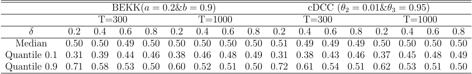
settings are the same with those studied in the bivariate case except for the replications, which are reduced to 2000. Figure 4.2 plots the empirical rejection rates of ˆMT(2) for small and large samples. There are two nontrivial observations. First, the test gains more powers even in small samples. This makes sense as the order of CUSUM statistics depends on ¯d according to Remark 2.1 in Aue et al. (2009). Consequently, Table 4.2 reports the more accurate estimation of t∗. Second, the test looks slightly over–sized. We attribute this distortion to the finite
sample bias of the Gaussian QMLE estimator in multivariate GARCH models. Note that the consistency of Gaussian QMLE works under strict stationarity condition, the near–integrate higher dimensional processes generated in our simulations might produce more outliers. Hence the QMLE estimators might not be accurate for small sample sizes. A similar issue has been discussed in Boudt and Croux (2010).
Table 4.2. Empirical performance of t∗
T, the estimator for t
∗
=T /2, when d= 9
BEKK(a= 0.2&b= 0.9) cDCC (θ2= 0.01&θ3 = 0.95)
T=300 T=1000 T=300 T=1000
δ 0.2 0.4 0.6 0.8 0.2 0.4 0.6 0.8 0.2 0.4 0.6 0.8 0.2 0.4 0.6 0.8
Median 0.50 0.50 0.50 0.50 0.50 0.50 0.50 0.50 0.50 0.50 0.50 0.50 0.50 0.50 0.50 0.50 Quantile 0.1 0.43 0.48 0.49 0.49 0.49 0.50 0.50 0.50 0.43 0.46 0.48 0.49 0.48 0.50 0.50 0.50 Quantile 0.9 0.56 0.51 0.50 0.50 0.52 0.50 0.50 0.50 0.57 0.51 0.50 0.50 0.52 0.51 0.50 0.50
5. An empirical application: testing for financial contagion
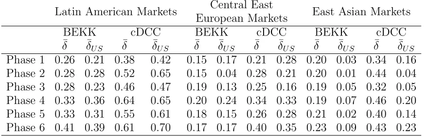
[image:10.612.72.557.529.610.2]We collect three groups of emerging stock market price indexes in three regions: six Latin Ameri-can markets including Argentina (Argentina MERVAL), Brazil (Brazil BOVESPA), Chile (Chile Santiago SE General), Mexico (Mexico IPC), Colombia (Colombia IGBC), Peru (BVL Gen-eral); seven Central East European (CEE hereafter) markets including Czech (Prague SEPX), Estonia (OMX Tallin), Hungary (Budapest), Poland (Warsaw General), Romania (Romania BET), Slovakia (Slovakia SAX 16), Slovenia (Slovenian blue chip); nine East Asian markets including Hong Kong (Hang Seng), Indonesia (IDX composite), South Korea (Korea SE com-posite), Malaysia (Malaysia KLCI), Philippines (Philippine SE), Singapore (Straits Times), Taiwan (Taiwan SE weighted), Thailand (Bangkok S.E.T), China (Shanghai S.E. A share). The S&P 500 index of the United States is used as the eye of the storm for each group. The Germany index (DAX 40) and the Japan index (Nikki 225) are also collected due to their im-portant influence on CEE and East Asian countries, respectively. The data are taken from the Datastream database and cover the period going from the 1st of September 2006 to the 1st of September 2010. We calculate log returns for each index to achieve the mean stationarity. To find changes in the correlation structures of these three data sets, we use ˆMT(2) in the BEKK as well as in the cDCC models. If a change is detected, we estimate the time of change and split the data into two subsets at the estimated time of change. Then we look for changes in both subsets (binary segmentation). Thus we segment the data into 6 homogeneous subsets. The change–point detection results are displayed in Figure 5.1. Overall, both models show con-sistent patterns. The correlation structures initially changed around February 2007 (Chinese stock bubble) and then changed around August 2007 (ceasing activities in the U.S. mortgage debt market), the third change happened close to September 2008 (the bankruptcy of Lehman Brothers), and the fourth and fifth changes occurred in the second half of 2009 (bailout decision made by G20 summit) and April 2010 (European debt crisis), respectively. Basically, these five dates split the whole sample into six periods: boom, panic, bubble, bust, recovery and new cri-sis. The reactions to crises are faster in the Latin American region because of the higher level of integration with U.S. The capital flow from the U.S. has less impact on CEE markets due to the regional economic dominance by Germany. The banking systems in the CEE countries are largely dominated by U.S. and Western European banks/financial institutions, mainly German banks. Beside the direct falling in their capital flows with U.S. banks, the German authority, as a regional dominance, would implement appropriate policies to resist market risks during the crisis, thereby providing an indirect buffer zone to CEE countries. East Asian markets are relatively less connected with the U.S. and tend to have higher resistance, which might be explained with their closer relation with the large economies in the area, such as Japan and China.
during the European debt crisis. These results imply that contagion effects are significant in all data sets, resulting a higher integrated but more fragile global capital market.
Figure 5.1. Plots of the conditional correlations between the U.S. and Latin American (left column), CEE (middle column), Asian (right column) in the BEKK (first row) and cDCC (second row) models. The vertical lines are the estimated times of changes.
Year
Sep.2006 May.2007 Jan.2009 Sep.2008 May.2009 Jan.2010 Sep.2010
Value -0.4 -0.2 0 0.2 0.4 0.6 0.8 1
1.2 Conditional Correlations between US and Latin American markets(BEKK)
(Argentina) (Brazil) (Chile) (Mexico) (Colombia) (Peru) Year
Sep.2006 May.2007 Jan.2009 Sep.2008 May.2009 Jan.2010 Sep.2010
Value -0.4 -0.2 0 0.2 0.4 0.6 0.8 1
1.2 Conditional Correlations between US and Central East European markets(BEKK)
(Czech) (Estonia) (Hungary) (Poland) (Romania) (Slovakia) (Slovenia) Year
Sep.2006 May.2007 Jan.2009 Sep.2008 May.2009 Jan.2010 Sep.2010
Value -0.4 -0.2 0 0.2 0.4 0.6 0.8 1
1.2 Conditional Correlations between US and East Asian markets(BEKK)
(Hong Kong) (Indonesia) (Japan) (South Korea) (Malaysia) (Philippines) (Singapore) (Taiwan) (Thailand) (China) Year
Sep.2006 May.2007 Jan.2009 Sep.2008 May.2009 Jan.2010 Sep.2010
Value -0.4 -0.2 0 0.2 0.4 0.6 0.8 1
1.2 Conditional Correlations between US and Latin American markets(cDCC)
(Argentina) (Brazil) (Chile) (Mexico) (Colombia) (Peru) Year
Sep.2006 May.2007 Jan.2009 Sep.2008 May.2009 Jan.2010 Sep.2010
Value -0.4 -0.2 0 0.2 0.4 0.6 0.8 1
1.2 Conditional Correlations between US and Central East European markets(cDCC)
(Czech) (Estonia) (Hungary) (Poland) (Romania) (Slovakia) (Slovenia) Year
Sep.2006 May.2007 Jan.2009 Sep.2008 May.2009 Jan.2010 Sep.2010
Value -0.4 -0.2 0 0.2 0.4 0.6 0.8 1
1.2 Conditional Correlations between US and East Asian markets(cDCC)
(Hong Kong) (Indonesia) (Japan) (South Korea) (Malaysia) (Philippines) (Singapore) (Taiwan) (Thailand) (China)
Table 5.1. The regional correlation levels and correlation levels with the U.S. market between 2006 and 2010
Latin American Markets Central East
European Markets East Asian Markets
BEKK cDCC BEKK cDCC BEKK cDCC
¯
δ δ¯U S δ¯ δ¯U S δ¯ δ¯U S δ¯ δ¯U S δ¯ δ¯U S δ¯ δ¯U S
Phase 1 0.26 0.21 0.38 0.42 0.15 0.17 0.21 0.28 0.20 0.03 0.34 0.16 Phase 2 0.28 0.28 0.52 0.65 0.15 0.04 0.28 0.21 0.20 0.01 0.44 0.04 Phase 3 0.28 0.23 0.46 0.47 0.19 0.13 0.25 0.16 0.19 0.05 0.32 0.05 Phase 4 0.33 0.36 0.64 0.65 0.20 0.24 0.34 0.33 0.19 0.07 0.46 0.20 Phase 5 0.33 0.31 0.55 0.61 0.18 0.15 0.26 0.28 0.21 0.02 0.40 0.14 Phase 6 0.41 0.39 0.61 0.70 0.17 0.17 0.40 0.35 0.23 0.09 0.43 0.23
6. Conclusion
[image:12.612.96.535.417.557.2]the U.S.. The findings indicated that there were global contagion effects and resulted a more fragile global capital market.
It is worth noticing that, although our test is valid for models which asymmetry in the dynamics of conditional variance such as the cDCC model, a generalization to all asymmetric multivariate GARCH processes is not made here, but it will definitely be an object of future research. The main issue to overcome is that so far, there are only few theoretical results available on the consistency of estimators for stationary asymmetric multivariate GARCH processes. The gen-eral methods in Meyn and Tweedie (1993) can be in theory used, but it is clear from Boussama et al. (2011) and Fermanian and Malongo (2017) that the calculations will be lengthy using methods and results from probability theory and algebraic geometry. The parameters could be estimated by the QMLE. If dimension d is large, then a large number of parameters need to be estimated, however the variance targeting estimators could help to overcome numerical issues. As in Aue et al. (2009), the limits in Theorem 2.2 might be approximated well in case of moderate and large d. Also, detecting change points in conditional correlation structure with the non-zero conditional mean might be another subject of further research.
Appendix A. Proofs of Theorems 2.1 and 2.2
We start with the weak convergence of the process s(t),0≤t ≤T.
Lemma A.1. If H0 and Assumptions 2.1–2.5 are satisfied, then we have
T−1/2(s(T u)−Es(T u)) D
¯ d
[0,1]
−→ WD(u),
where WD(u),0≤ u≤1 is a Brownian motion in R
¯
d with covariance matrix D, i.e. W(u) is
Gaussian with EW(u) =0 and EWD(u)W⊤D(v) = min(u, v)D.
Proof. It follows from Assumptions 2.1–2.4 thaty∗
t(i)y∗(j) is also stationary andβ–mixing with the same rate as of yt. Also, since Assumption 2.3 implies thatτt(i)≥τ0 we get that
E|y∗
t(i)y
∗
t(j)|r/2 ≤ 1
τ2
0
(E|y∗
t(i)|rE|y
∗
t(j)|r)1/2 <∞
via the Cauchy–Schwartz inequality and the moment condition in Assumption 2.4. Hence the result of Ibragimov (1962) (cf. also Rio, 2000) implies the lemma.
Proof of Theorem 2.1. Lemma A.1 implies that
(A.1) T−1/2
s(T u)−⌊T u⌋
T s(T)
Dd¯
[0,1]
−→ WD(u)−uWD(1).
Checking the covariance structure, one can easily verify that
D−1/2(W
D(u)−uWD(1)),0≤u≤1
(A.2)
D
={(B1(u), B2(u), . . . , Bd¯(u)),0≤u≤1},
whereB1, B2, . . . , Bd¯are independent Brownian bridges. Hence Theorem 2.1 follows from (A.1)
and (A.2) via the continuous mapping theorem.
Proof of Theorem 2.2. It follows from the definition of ˆyt(i) that
ˆ
yt(i)ˆyt(j)−yt∗(i)y
∗
at,1(i, j) =yt(i)yt(j)
1 ¯
τt(i; ˆθT)
− 1
τt(i; ˆθT)
!
1 ¯
τt(j; ˆθT)
− 1
τt(j; ˆθT)
!
,
at,2(i, j) =yt(i)yt(j)
1 ¯
τt(i,θˆT)
− 1
τt(i,θˆT)
!
1
τt(j; ˆθT)
− 1
τt(j;θ0)
!
,
at,3(i, j) =yt(i)
1 ¯
τt(i,θˆT)
− 1
τt(i,θˆT)
!
yt(j)
τt(i),
at,4(i, j) =yt(i)yt(j)
1
τt(i; ˆθT)
− 1
τt(i;θ0)
!
1 ¯
τt(j; ˆθT)
− 1
τt(j; ˆθT)
!
,
at,5(i, j) =yt(i)yt(j)
1
τt(i; ˆθT)
− 1
τt(i;θ0)
!
1
τt(j; ˆθT)
− 1
τt(j;θ0)
!
,
at,6(i, j) =
yt(i)
τt(i)yt(j)
1 ¯
τt(j; ˆθT)
− 1
τt(j; ˆθT)
!
,
at,7(i, j) =yt(i)
1
τt(i; ˆθT)
− 1
τt(i;θ0)
!
yt(j)
τt(j),
at,8(i, j) =
yt(i)
τt(i)yt(j)
1
τt(j; ˆθT)−
1
τt(j;θ0)
!
.
Since ¯τt(i,θˆT)τ0 >0, by Assumptions 2.7 and 2.6 we have on account of the mean value theorem
that
T−1/2 max
1≤t≤T
t
X
s=1
|as,1|=OP(1)T−1/2 T
X
t=1
|yt(i)yt(j)|a2(t).
We can assume without loss of generality that a(t) is non increasing as t → ∞. Using again Assumption 2.6 we can find a sequence aT such that T−1/2aT → 0 and T1/2a(aT) → 0 and therefore
T−1/2
T
X
t=1
|yt(i)yt(j)|a2(t) (A.3)
≤T−1/2
aT X
t=1
|yt(i)yt(j)|a2(t) +T−1/2
T
X
t=aT+1
|yt(i)yt(j)|a2(t)
=OP(T−1/2aT +T1/2a2(aT)) =oP(1),
where we used the ergodic theorem that
1
L
L
X
t=1
since by Assumption 2.4E|y0(i)y0(j)| ≤(Ey02(i)Ey02(j))1/2 <∞. Putting together Assumptions
2.6–2.8 we conclude via two term Taylor expansion and the mean value theorem that
T−1/2 max
1≤t≤T
t
X
s=1
|as,2|=OP(T−1/2) T
X
t=1
|yt(i)yt(j)|a(t)
h
kgt(j)kkθˆT −θk+ ¯gtkθˆT −θ0k2
i
.
Following the proof of (A.3) one can show that
T−1/2
T
X
t=1
|yt(i)yt(j)|a(t)kgt(j)kkθˆT −θ0k=OP(1) 1
T
T
X
t=1
|yt(i)yt(j)|a(t)kgt(j)k=oP(1),
since E|yt(i)yt(j)|kgt(j)k ≤ (E|yt(i)yt(j)|2Ekgt(j)k2)1/2 ≤ (Eyt4(i)Eyt4(j))1/4(Ekgt(j)k2)1/2 <
∞. The same arguments give
T−1/2
T
X
t=1
|yt(i)yt(j)|a(t)¯gtkθˆT −θ0k2 =OP(1) 1
T3/2
T
X
t=1
|yt(i)yt(j)|a(t)¯gt
=OP(1)
1
T1/2 1max≤t≤Tg¯t
1 T T X t=1
|yt(i)yt(j)|a(t) = oP(1),
since Eg¯2
0 <∞ implies max1≤t≤T g¯t=oP(T1/2). Similarly,
T−1/2 max
1≤t≤T
t
X
s=1
|as,3|=OP(1)T−1/2 T
X
t=1
|yt(i)yt(j)|a(t) = oP(1)
and by symmetry, T−1/2max
1≤t≤T Pts=1|as,ℓ|=oP(1), ℓ= 4,5,6. Assumption 2.8 implies that
T−1/2 max
1≤t≤T
t X s=1
as,7−
t
X
s=1
yt(i)
τ2
t(i)
yt(j)
τt(j)gs(i)
⊤
(θ0 −θˆT)
=OP(1)T−1/2 T
X
s=1
|yt(i)yt(j)|¯gtkθ0−θˆTk2 =OP(1)
T−1/2 max
1≤t≤Tg¯t
1 T T X s=1
|yt(i)yt(j)|=oP(1).
Using again the ergodic theorem and Assumption 2.4, we conclude
T−1/2 max
1≤t≤T
t X s=1
ys(i)
τ2
s(i)
ys(j)
τs(j)gs(i)−
t T
T
X
s=1
ys(i)
τ2
s(i)
ys(j)
τs(j)gs(i)
!⊤
(θ0−θˆT)
=OP(1) 1
T 1max≤t≤T
t X s=1
ys(i)
τ2
s(i)
ys(j)
τs(j)gs(i)−
t T
T
X
s=1
ys(i)
τ2
s(i)
ys(j)
τs(j)gs(i)
=oP(1)
since E|y0(i)y0(j)|kg0(i)k<∞. Hence we obtain that
T−1/2 max
1≤t≤T
t X s=1
as,7−
t T
T
X
s=1
as,7
=oP(1)
and by the same arguments
T−1/2 max
1≤t≤T
t X s=1
as,8−
t T
T
X
s=1
as,8
Thus we proved that
T−1/2 max
1≤t≤T
t
X
s=1
ˆ
ys(i)ˆys(j)−⌊t⌋
T
T
X
s=1
ˆ
ys(i)ˆys(j)
!
−
t
X
s=1
y∗
s(i)y
∗
s(j)−
t T
T
X
s=1
y∗
s(i)y
∗
s(j)
!
=oP(1),
and therefore the result follows from Theorem 2.1.
Acknowledgements. We are grateful to Professors Christian Francq and Jean–Michel Zakoian for their comments on the first version of this paper and for useful references. We also thank the editor, Todd Clark, the associate editor and two anonymous referees, whose detailed and constructive comments helped to improve the quality of the paper.
References
[1] Aielli, G.P.: Dynamic conditional correlation: on properties and estimation. Journal of Business and
Economic Statistics31(2013), 282–299.
[2] Andreou, E. and Ghysels, E.: Detecting multiple breaks in financial market volatility dynamics.Journal of
Applied Econometrics17(2002), 579–600.
[3] Andreou, E. and Ghysels, E.: Tests for breaks in the conditional co-movements of asset returns. Statistica
Sinica(2003), 1045–1073.
[4] Aue, A., H¨ormann, S., Horv´ath, L., and Reimherr, M.: Break detection in the covariance structure of multivariate time series models.The Annals of Statistics37(2009), 4046–4087.
[5] Aue, A. and Horv´ath, L.: Structural breaks in time series.Journal of Time Series Analysis34(2013), 1–16. [6] Bai, J. and Perron, P.: Estimating and testing linear models with multiple structural changes.Econometrica
66(1998), 47–78.
[7] Bauwens, L., Laurent, S. and Rombouts, J.V.K.: Multivariate GARCH models: A survey.Journal of Applied
Econometrics21(2006), 79-109.
[8] Blatt, D., Candelon, B. and Manner, H.: Detecting contagion in a multivariate time series system: An application to sovereign bond markets in Europe.Journal of Banking & Finance59(2015), 1–13.
[9] Bollerslev, T.: Modelling the coherence in short–run nominal exchange rates: a multivariate generalized ARCH model.The Review of Economics and Statistics(1990), 498–505.
[10] Boudt, K., Croux, C.: Robust M-estimation of multivariate GARCH models. Computational Statistics &
Data Analysis(2010), 2459-2469.
[11] Boussama, F., Fuchs, F. and Stelzer, R.: Stationarity and geometric ergodicity of BEKK multivariate GARCH models.Stochastic Processes and Their Applications121(2011), 2331–2360.
[12] Cappiello, L, Engle, R.F. and Sheppard, K.: Asymmetric dynamics in the correlations of global equity and bond returns.Journal of Financial Econometrics 4(2006), 537–572.
[13] Comte, F. and Lieberman, O.: Asymptotic theory for multivariate GARCH processes.Journal of
Multi-variate Analysis84(2003), 61-84.
[14] Cs¨org˝o, M. and Horv´ath, L.: Limit Theorems in Change–point Analysis.Wiley, 1997.
[15] Demetrescu, M. and Wied, D.: Residual–based inference on moment hypotheses, with an application to
testing for constant correlation.Discussion paper, Nr. 37/2016, University of Dortmund.
[16] De Pooter, M. and Van Dijk, D.: Testing for changes in volatility in heteroskedastic time series–a further examination.Technical report, Econometrics Institute Research Papers(2004).
[17] Dimitriou, D., Kenourgios, D. and Simos, T.: Global financial crisis and emerging stock market contagion: a multivariate FIAPARCH–DCC approach.International Review of Financial Analysis30(2013), 46–56. [18] Dungey, M., Milunovich, G., Thorp, S. and Yang, M.: Endogenous crisis dating and contagion using smooth
transition structural GARCH.Journal of Banking & Finance58 (2015), 71–79.
[19] Engle, R.F.: Dynamic conditional correlation: A simple class of multivariate generalized autoregressive conditional heteroskedasticity models.Journal of Business & Economic Statistics20(2002), 339–350. [20] Engle, R.F:Anticipating Correlations: A New Paradigm for Risk Management. Princeton University Press,
[21] Engle, R.F. and Kroner, K.F.: Multivariate simultaneous generalized ARCH. Econometric Theory
11(1995), 122-150.
[22] Fermanian, J.-D. and Malongo, H.: On the stationarity of dynamical conditional correlation models.
Econo-metric Theory33(2017), 636–663.
[23] Forbes, K.J. and Rigobon, R.: No contagion, only interdependence: measuring stock market comovements.
The journal of Finance57(2002), 2223–2261.
[24] Francq, C. and Horv´ath, L. and Zakoian, J.M.: Variance targeting estimation of multivariate GARCH models.Journal of Financial Econometrics 14(2016), 353–382.
[25] Francq, C. and Zakoian, J.M.: GARCH Models.Wiley, 2010.
[26] Fryzlewicz, P. and Rao, S.S.: Mixing properties of ARCH and time–varying ARCH processes, Bernoulli
17(2011), 320–346.
[27] Hafner, C.M. and Preminger, A.: On asymptotic theory for multivariate GARCH models. Journal of
Multivariate Analysis100(2009), 2044–2054.
[28] Horv´ath, L. and Rice, G.: Extensions of some classical methods in change point analysis (with discussions).
TEST23(2014), 219–290.
[29] Inclan, C. and Tiao, G.C.: Use of cumulative sums of squares for retrospective detection of changes of variance.Journal of the American Statistical Association89(1994), 913–923.
[30] Kokoszka, P. and Leipus, R.: Change–point estimation in ARCH modelsBernoulli6(2000), 513–539. [31] Kulperger, R. and Yu, H.: High moment partial sum processes of residuals in GARCH models and their
applications.Annals of Statistics33(2005), 2395–2422.
[32] Lavielle, M. and Teyssi´ere, G.: Detection of multiple change–points in multivariate time series.Lithuanian
Mathematical Journal46(2006), 287–306.
[33] Lee, S., Na, O. and Na, S.: On the cusum of squares test for variance change in nonstationary and nonparametric time series models. The Annals of the Institute of Statistical Mathematics 55(2003), 467– 485.
[34] Ling, S.: Testing for change points in time series models and limiting theorems for NED sequences.Annals
of Statistics35(2007), 1213–1237.
[35] Meyn, S.P. and Tweedie, R.L.: Markov Chains and Stochastic Stability.Springer, London, 1993.
[36] Pedersen, R.S. and Rahbek, A.: Multivariate variance targeting in the BEKK–GARCH model.
Economet-rics Journal17(2014), 24–55.
[37] Qu, Z. and Perron, P.: Estimating and testing structural changes in multivariate regressions.Econometrica
75(2007) 459–502.
[38] Silvennoinen, A. and Ter¨asvirta, T.: Multivariate GARCH models. In: Handbook of Financial Time Series
(Davis, R.A., Kreiss, J.-P. and Mikosch, T., Eds.), Springer, New York, 2009.
[39] Wied, D., Kr¨amer, W. and Dehling, H.: Testing for a change in correlation at an unknown point in time using an extended functional delta method.Econometric Theory28(2012), 570–589.
Online Supplement
Appendix B. Verification of the conditions of Theorem 2.2 for the BEKK
model (Example 3.1)
According to Boussama et al. (2011), we assume
Assumption B.1. The distribution of et is absolutely continuous with respect to the Lebesgue
measure on Rd and the point zero is an interior point of the support of the distribution of e
t
and
Assumption B.2. The spectral radius of A+B is less than 1.
Boussama et. al. (2011) contains a detailed proof that (2.1) and (3.1) have a unique, stationary, ergodic and geometrically β–mixing solution (They also point out that if there is a stationary solution, then Assumption B.2 must hold). Hence, Assumptions 2.2 holds and by (3.1) we also have Assumption 2.3 with Σ0 = C. The mixing requirement in Assumption 2.4 holds and
we only need to assume that kytkr <∞ (We note that Hafner and Preminger (2009) provide explicit conditions for the existence of moments). If Assumption 2.5 holds, then the mixing property ofytand the existence of the moments ofytyield Assumption 2.9 along the lines of the calculations in Wu and Zaffaroni (2018). The parameters of the BEKK model can be estimated by the QMLE and the variance targeting QMLE. Hafner and Preminger (2009), Pedersen and Rahbek (2014) and Francq et al. (2016) establish Assumption 2.6 withρt with some 0< ρ <1, and the established asymptotic normality in those papers yields Assumption 2.7. Finally, the computation of the second derivatives of τt(i,θ) in Pedersen and Rahbek (cf. also Hafner and Preminger, 2009 and Francq et al. 2016) gives Assumption 2.8.
Appendix C. Verification of the conditions of Theorem 2.2 for the cDCC
model (Example 3.2)
Aielli (2013) points out that since C is positive definite and θ1 > 0, θ2 > 0, θ1 +θ2 < 1, the
cDCC sequences have the properties of existence, uniqueness and ergodicity, if the univariate GARCH process defined by hi(ζi,· · ·) have these properties. Carrasco and Chen (2002) and H¨ormann (2008) assume thatht,i =hi(ζi, yt−1(i), yt−2(i), . . .) satisfyht(i) =ui(vt(i)) with some
2.6–2.8. The proofs in Section 3.3 in Aielli (2013) yield that the estimators obtained in the second and third steps have the properties in Assumptions 2.6–2.8.
Appendix D. Further examples for time dependent conditional volatilities
In this section we consider several other models where Assumptions 2.1–2.9 are satisfied. There are two main methods to establish stationarity and geometric mixing properties of non–linear time series models. Markov chain theory combined with algebraic geometry can be used to establish the existence and basic properties of the underlying model. Important technical tools are summarized in the reference book of Meyn and Tweedie (1993). Diaconis and Freedman (1999) showed that random recursions satisfying “contraction in average” have a unique sta-tionary solution and the method of the proof gives geometric ergodicity. Applications of the method of Diaconis and Freedman (1999) to non–linear time series are detailed in Douc et al. (2014).
Example D.1. (CCC(p, q) model) Bollerslev (1990) and Jeantheau (1998) specified the con-stant conditional correlation model by the following equations:
(D.1) Σt =DtRDt,
(D.2) Dt= diag(τt(1), τt(2), . . . , τt(d)), ht= (τt2(1), τt2(2), . . . , τt2(d))
⊤
,
and
(D.3) ht=c+ q
X
ℓ=1
Aℓ(yt−ℓ◦yt−ℓ) +
p
X
j=1
Bjht−j,
where ◦ denotes the Hadamard product of vectors (coordinate wise multiplication), R is a correlation matrix,cis a vector of positive coordinates,Aℓ,1≤ℓ≤q,Bj,1≤j ≤pare matrices with nonnegative elements. Sufficient conditions for the existence of a unique stationary solution and existence of moments are given in Aue et al. (2009) and their method can also be used to prove (2.4). For further discussion we refer to Francq and Zakoian (2010). Francq and Zakoian (2010) also gave a detailed account of the estimation of the parameters of an CCC(p, q) sequence by quasi maximum likelihood and Assumptions 2.6–2.8 are established. In addition to the QMLE, the variance targeting estimator also satisfies our assumptions (cf. Francq et al., 2016). Francq and Zakoian (2014) proposed a new method to estimate parameters utilizing the covariance structure of the observations. Their proofs show that Assumptions 2.6–2.8 hold.
Example D.2. (DCC-GARCH model) Dynamic conditional correlation GARCH models are an extension of the cDCC and CCC models of Examples 3.2 and D.1. It is assumed that (3.2) and (3.3) hold but Equation (3.4) is replaced by
(D.4) Qt=C+Ay∗t−1(y
∗
t−1)
⊤
A⊤+BQt−1B,
where C is a positive definite matrix, A and B are d×d matrices. Fermanian and Malongo (2017) provide general conditions for the existence of a unique stationary and ergodic solution of the DCC equations. Their proofs yield Assumption 2.4. It follows from the definition of DCC that Assumptions 2.2 and 2.3 hold. Pape et al. (2017) discuss the special case when
C,A and B are real numbers. They also provide estimators for the parameters which satisfy Assumptions 2.6–2.8.
Example D.3. (Factor model) Engle, Ng and Rothschild (1990) defined the conditional co-variance matrix Σt by
Σt=C+ p
X
j=1
λt(j)βjβ⊤j and λt(j) = ωj+αjyt2−1(j) +βjλt−1(j),
where Cis a positive definite matrix, ωj >0, αj ≥0, βj ≥0,1≤ j ≤p, and β1,β2, . . . ,βp are linearly independent vectors. Francq and Zakoian (2010) pointed out that the factor model can be written in a BEKK form, so clearly Assumptions 2.1–2.9 are satisfied under mild conditions.
For further multivariate GARCH type models we refer to the survey papers of Bauwens et al. (2006) and Silvennoinen and Ter¨asvirta (2009).
Appendix E. Further Monte Carlo Simulations
We extend the Monte Carlo simulations in Section 4 to Examples D.1 - D.3. We list the specifications for the examples next. As before, d = 2 (bivariate observations), p = 1 and
q = 1 in Examples D.1, the magnitude of the change is δ, δ = 0 is the null hypothesis and under the alternative the change from 0 to δ at t∗
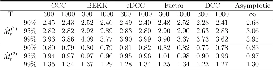
[image:20.612.85.542.379.497.2]= T /2. For comparison we report critical values in Table E.1 for all examples. Table E.1 shows that the asymptotic critical values mildly overestimate the empirical ones.
Table E.1. Critical Values for the statistics ˆMT(1), ˆMT(2) statistics (d=2) and the asymptotic critical values computed from the distribution ofM(1)andM(2)(d=2)
CCC BEKK cDCC Factor DCC Asymptotic T 300 1000 300 1000 300 1000 300 1000 300 1000 ∞
ˆ
Mt(1)
90% 2.45 2.43 2.52 2.46 2.49 2.40 2.48 2.52 2.28 2.41 2.63 95% 2.82 2.82 2.92 2.89 2.83 2.80 2.90 2.90 2.63 2.83 3.06 99% 3.96 3.86 4.09 3.77 3.90 3.99 3.90 3.67 3.73 3.62 3.95
ˆ
Mt(2)
90% 0.80 0.79 0.80 0.79 0.81 0.82 0.82 0.82 0.75 0.78 0.83 95% 0.94 0.97 0.97 0.96 0.95 0.96 1.01 0.98 0.90 0.96 0.97 99% 1.35 1.34 1.37 1.29 1.28 1.34 1.35 1.34 1.23 1.27 1.30
E.1. Constant Conditional Correlations (CCC).
The constant correlation matrix R is
(E.1) R=
1 δ
δ 1
To set Dt, we set c= (0.01,0.01)⊤,
(E.2) A1 =
a 0
0 a
and B1 =
b 0
0 b
with a = 0.02 and b = 0.94 in our simulation study. The choice of A1 and B1 is motivated by
the empirical observation that financial data show low ARCH but high GARCH (persistence) effect. The matrices A1 and B1 determine the dynamics of the process, but their values are
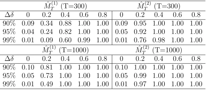
of the change as the percentage of the observations. The estimator is rather accurate and it is improving asδ and/orT are increasing.
Table E.2. Empirical rejection rates for ˆMT(1) and ˆMT(2) in the CCC model of Example D.1
ˆ
MT(1) (T=300) MˆT(2) (T=300) ∆δ 0 0.2 0.4 0.6 0.8 0 0.2 0.4 0.6 0.8 90% 0.09 0.34 0.88 1.00 1.00 0.09 0.95 1.00 1.00 1.00 95% 0.04 0.24 0.82 1.00 1.00 0.05 0.92 1.00 1.00 1.00 99% 0.01 0.09 0.60 0.99 1.00 0.01 0.76 0.98 1.00 1.00
ˆ
[image:21.612.152.474.433.507.2]MT(1) (T=1000) MˆT(2) (T=1000) ∆δ 0 0.2 0.4 0.6 0.8 0 0.2 0.4 0.6 0.8 90% 0.10 0.81 1.00 1.00 1.00 0.10 1.00 1.00 1.00 1.00 95% 0.05 0.73 1.00 1.00 1.00 0.05 0.99 1.00 1.00 1.00 99% 0.01 0.49 1.00 1.00 1.00 0.01 0.97 1.00 1.00 1.00
Table E.3. Estimated of the time of change as a percentage of the observation period in the CCC model of Example D.1 when t∗ =T /2
T=300 T=1000
∆δ 0.2 0.4 0.6 0.8 0.2 0.4 0.6 0.8 Median 0.50 0.49 0.49 0.49 0.50 0.50 0.50 0.50 Quantile 0.1 0.31 0.40 0.45 0.47 0.41 0.47 0.48 0.49 Quantile 0.9 0.70 0.57 0.52 0.50 0.60 0.52 0.50 0.50
E.2. Dynamic Conditional Correlations (DCC-GARCH).
Following the DGP D.4, we use C=R of (E.1), and set the coefficient matrices A and B,
A=
a 0.001
0.001 a
, B =
b 0.01
0.01 b
Table E.4. Empirical rejection rates for ˆMT(1) and ˆMT(2) in the DCC-GARCH model of Example D.2
T=300
a= 0.01 &b= 0.9 a= 0.01 &b= 0.95
ˆ
MT(1) MˆT(2) MˆT(1) MˆT(2)
δ 0 0.2 0.4 0.6 0.8 0 0.2 0.4 0.6 0.8 0 0.2 0.4 0.6 0.8 0 0.2 0.4 0.6 0.8 90% 0.11 0.41 0.90 1.00 1.00 0.11 0.99 1.00 1.00 1.00 0.12 0.40 0.84 1.00 1.00 0.13 0.96 1.00 1.00 1.00 95% 0.06 0.29 0.84 1.00 1.00 0.06 0.95 1.00 1.00 1.00 0.07 0.29 0.78 0.99 1.00 0.07 0.93 0.99 1.00 1.00 99% 0.01 0.11 0.58 0.98 1.00 0.02 0.83 0.99 1.00 1.00 0.02 0.12 0.55 0.94 1.00 0.02 0.85 0.97 1.00 1.00
a= 0.02 &b= 0.9 a= 0.02 &b= 0.95
ˆ
MT(1) MˆT(2) MˆT(1) MˆT(2)
δ 0 0.2 0.4 0.6 0.8 0 0.2 0.4 0.6 0.8 0 0.2 0.4 0.6 0.8 0 0.2 0.4 0.6 0.8 90% 0.14 0.40 0.85 1.00 1.00 0.14 0.97 1.00 1.00 1.00 0.16 0.36 0.73 0.98 1.00 0.16 0.97 1.00 1.00 1.00 95% 0.07 0.30 0.78 0.99 1.00 0.07 0.94 0.99 1.00 1.00 0.10 0.26 0.65 0.96 1.00 0.08 0.93 0.99 1.00 1.00 99% 0.01 0.12 0.53 0.95 1.00 0.02 0.83 0.98 1.00 1.00 0.02 0.10 0.41 0.86 0.99 0.02 0.81 0.97 1.00 1.00
T=1000
a= 0.01 &b= 0.9 a= 0.01 &b= 0.95
ˆ
MT(1) MˆT(2) MˆT(1) MˆT(2)
δ 0 0.2 0.4 0.6 0.8 0 0.2 0.4 0.6 0.8 0 0.2 0.4 0.6 0.8 0 0.2 0.4 0.6 0.8 90% 0.12 0.80 1.00 1.00 1.00 0.12 1.00 1.00 1.00 1.00 0.14 0.78 1.00 1.00 1.00 0.15 1.00 1.00 1.00 1.00 95% 0.05 0.69 1.00 1.00 1.00 0.06 0.99 1.00 1.00 1.00 0.07 0.67 1.00 1.00 1.00 0.07 0.99 1.00 1.00 1.00 99% 0.01 0.51 1.00 1.00 1.00 0.01 0.97 1.00 1.00 1.00 0.02 0.46 1.00 1.00 1.00 0.02 0.96 1.00 1.00 1.00
a= 0.02 &b= 0.9 a= 0.02 &b= 0.95
ˆ
MT(1) Mˆ
(2)
T Mˆ
(1)
T Mˆ
(2) T
[image:22.612.73.556.441.582.2]δ 0 0.2 0.4 0.6 0.8 0 0.2 0.4 0.6 0.8 0 0.2 0.4 0.6 0.8 0 0.2 0.4 0.6 0.8 90% 0.15 0.73 1.00 1.00 1.00 0.16 1.00 1.00 1.00 1.00 0.17 0.68 1.00 1.00 1.00 0.17 0.99 1.00 1.00 1.00 95% 0.07 0.64 1.00 1.00 1.00 0.07 0.99 1.00 1.00 1.00 0.08 0.57 0.98 1.00 1.00 0.07 0.98 1.00 1.00 1.00 99% 0.02 0.43 0.99 1.00 1.00 0.02 0.96 1.00 1.00 1.00 0.02 0.40 0.97 1.00 1.00 0.02 0.95 1.00 1.00 1.00
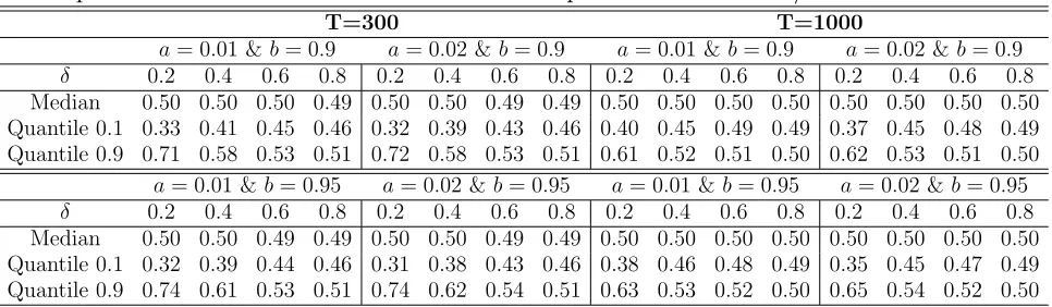
Table E.5. Estimation of the time of change as a percentage of the observation period in the DCC-GARCH model of Example D.2 when t∗ =T /2
T=300 T=1000
a= 0.01 &b= 0.9 a= 0.02 &b= 0.9 a= 0.01 &b= 0.9 a= 0.02 &b= 0.9
δ 0.2 0.4 0.6 0.8 0.2 0.4 0.6 0.8 0.2 0.4 0.6 0.8 0.2 0.4 0.6 0.8
Median 0.50 0.50 0.50 0.49 0.50 0.50 0.49 0.49 0.50 0.50 0.50 0.50 0.50 0.50 0.50 0.50 Quantile 0.1 0.33 0.41 0.45 0.46 0.32 0.39 0.43 0.46 0.40 0.45 0.49 0.49 0.37 0.45 0.48 0.49 Quantile 0.9 0.71 0.58 0.53 0.51 0.72 0.58 0.53 0.51 0.61 0.52 0.51 0.50 0.62 0.53 0.51 0.50
a= 0.01 &b= 0.95 a= 0.02 &b= 0.95 a= 0.01 &b= 0.95 a= 0.02 &b= 0.95
δ 0.2 0.4 0.6 0.8 0.2 0.4 0.6 0.8 0.2 0.4 0.6 0.8 0.2 0.4 0.6 0.8
Median 0.50 0.50 0.49 0.49 0.50 0.50 0.49 0.49 0.50 0.50 0.50 0.50 0.50 0.50 0.50 0.50 Quantile 0.1 0.32 0.39 0.44 0.46 0.31 0.38 0.43 0.46 0.38 0.46 0.48 0.49 0.35 0.45 0.47 0.49 Quantile 0.9 0.74 0.61 0.53 0.51 0.74 0.62 0.54 0.51 0.63 0.53 0.52 0.50 0.65 0.54 0.52 0.50
E.3. Factor-GARCH.
Let p = 2 in Example D.3. We use C = R of E.1. Let ω = 0.01, α1 = α2 = 0.01 (relatively
lower ARCH effect), β1 = β2 = 0.85, β1 = (0.85,0.85)⊤ or β1 = β2 = 0.95, β1 = (0.95,0.95)⊤
(high or very high persistence); α1 = α2 = 0.02 (relatively higher ARCH), β1 = β2 = 0.85,
β1 = (0.85,0.85)⊤
orβ1 =β2 = 0.95,β1 = (0.95,0.95)
⊤
(relatively lower or higher persistence), the conditional variances of the factors are generated recursively from λ0 = 1. The results are
Table E.6. Empirical rejection rates for ˆMT(1) and ˆMT(2) in the factor model of Example D.3
T=300
a= 0.01 &b= 0.85 a= 0.01 &b= 0.95
ˆ
MT(1)(T=300) MˆT(2)(T=300) MˆT(1)(T=300) MˆT(2)(T=300)
∆δ 0 0.2 0.4 0.6 0.8 0 0.2 0.4 0.6 0.8 0 0.2 0.4 0.6 0.8 0 0.2 0.4 0.6 0.8
90% 0.12 0.32 0.84 1.00 1.00 0.13 0.96 1.00 1.00 1.00 0.11 0.31 0.81 1.00 1.00 0.12 0.96 1.00 1.00 1.00 95% 0.06 0.21 0.74 0.99 1.00 0.06 0.91 1.00 1.00 1.00 0.06 0.19 0.70 0.99 1.00 0.06 0.91 0.99 1.00 1.00 99% 0.02 0.07 0.47 0.97 1.00 0.01 0.77 0.99 1.00 1.00 0.01 0.07 0.45 0.96 1.00 0.01 0.77 0.99 1.00 1.00
a= 0.02 &b= 0.85 a= 0.02 &b= 0.95
ˆ
MT(1)(T=300) MˆT(2)(T=300) MˆT(1)(T=300) MˆT(2)(T=300)
δ 0 0.2 0.4 0.6 0.8 0 0.2 0.4 0.6 0.8 0 0.2 0.4 0.6 0.8 0 0.2 0.4 0.6 0.8 90% 0.12 0.30 0.78 1.00 1.00 0.12 0.96 1.00 1.00 1.00 0.13 0.30 0.78 1.00 1.00 0.13 0.96 1.00 1.00 1.00 95% 0.06 0.20 0.66 0.99 1.00 0.05 0.90 1.00 1.00 1.00 0.06 0.20 0.66 0.99 1.00 0.06 0.91 1.00 1.00 1.00 99% 0.01 0.06 0.39 0.94 1.00 0.01 0.76 0.98 1.00 1.00 0.01 0.06 0.38 0.93 1.00 0.02 0.77 0.98 1.00 1.00
T=1000
a= 0.01 &b= 0.85 a= 0.01 &b= 0.95
ˆ
MT(1)(T=1000) MˆT(2)(T=1000) MˆT(1)(T=1000) MˆT(2)(T=1000)
δ 0 0.2 0.4 0.6 0.8 0 0.2 0.4 0.6 0.8 0 0.2 0.4 0.6 0.8 0 0.2 0.4 0.6 0.8 90% 0.12 0.70 1.00 1.00 1.00 0.13 1.00 1.00 1.00 1.00 0.12 0.69 1.00 1.00 1.00 0.13 1.00 1.00 1.00 1.00 95% 0.07 0.59 1.00 1.00 1.00 0.07 0.99 1.00 1.00 1.00 0.07 0.58 1.00 1.00 1.00 0.07 0.99 1.00 1.00 1.00 99% 0.02 0.40 1.00 1.00 1.00 0.02 0.95 1.00 1.00 1.00 0.02 0.39 1.00 1.00 1.00 0.01 0.95 1.00 1.00 1.00
a= 0.02 &b= 0.85 a= 0.02 &b= 0.95
ˆ
MT(1)(T=1000) Mˆ
(2)
T (T=1000) Mˆ
(1)
T (T=1000) Mˆ
(2)
[image:23.612.73.558.445.585.2]T (T=1000) δ 0 0.2 0.4 0.6 0.8 0 0.2 0.4 0.6 0.8 0 0.2 0.4 0.6 0.8 0 0.2 0.4 0.6 0.8 90% 0.13 0.67 1.00 1.00 1.00 0.14 1.00 1.00 1.00 1.00 0.14 0.65 1.00 1.00 1.00 0.14 1.00 1.00 1.00 1.00 95% 0.07 0.55 1.00 1.00 1.00 0.07 0.99 1.00 1.00 1.00 0.07 0.54 1.00 1.00 1.00 0.07 0.99 1.00 1.00 1.00 99% 0.02 0.35 0.99 1.00 1.00 0.02 0.95 1.00 1.00 1.00 0.02 0.34 0.99 1.00 1.00 0.02 0.95 1.00 1.00 1.00
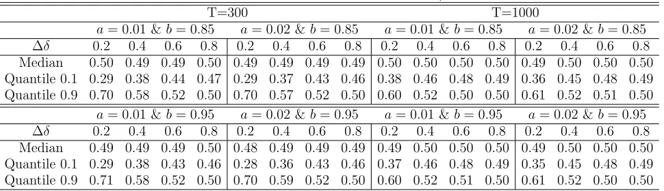
Table E.7. Estimation of the time of change as a percentage of the observation period in the factor model of Example D.3 whent∗
=T /2
T=300 T=1000
a= 0.01 &b= 0.85 a= 0.02 &b= 0.85 a= 0.01 &b= 0.85 a= 0.02 &b= 0.85 ∆δ 0.2 0.4 0.6 0.8 0.2 0.4 0.6 0.8 0.2 0.4 0.6 0.8 0.2 0.4 0.6 0.8 Median 0.50 0.49 0.49 0.50 0.49 0.49 0.49 0.49 0.50 0.50 0.50 0.50 0.49 0.50 0.50 0.50 Quantile 0.1 0.29 0.38 0.44 0.47 0.29 0.37 0.43 0.46 0.38 0.46 0.48 0.49 0.36 0.45 0.48 0.49 Quantile 0.9 0.70 0.58 0.52 0.50 0.70 0.57 0.52 0.50 0.60 0.52 0.50 0.50 0.61 0.52 0.51 0.50
a= 0.01 &b= 0.95 a= 0.02 &b= 0.95 a= 0.01 &b= 0.95 a= 0.02 &b= 0.95 ∆δ 0.2 0.4 0.6 0.8 0.2 0.4 0.6 0.8 0.2 0.4 0.6 0.8 0.2 0.4 0.6 0.8 Median 0.49 0.49 0.49 0.50 0.48 0.49 0.49 0.49 0.49 0.50 0.50 0.50 0.49 0.50 0.50 0.50 Quantile 0.1 0.29 0.38 0.43 0.46 0.28 0.36 0.43 0.46 0.37 0.46 0.48 0.49 0.35 0.45 0.48 0.49 Quantile 0.9 0.71 0.58 0.52 0.50 0.70 0.59 0.52 0.50 0.60 0.52 0.51 0.50 0.61 0.52 0.50 0.50
References
[1] Douc, R., Moulines, E. and Stoffer, D.S.: Nonlinear Time Series.CRC Press, Boca Raton, 2014.
[2] Engle, R. F. and Ng, V. K. and Rothschild, M.: Asset pricing with a factor-ARCH covariance structure: Empirical estimates for treasury bills.Journal of Econometrics 45(1990), 213–237.
[3] Francq, C. and Zakoian, J.M.: Comment on “Quasi–Maximum Likelihood Estimation of GARCH Models with Heavy Tailed Likelihoods” by J. Fan, L. Qi and D. Xiu. Journal of Business & Economic Statistics
[4] Jeantheau, T.: Strong consistency of estimators for multivariate ARCH models. Econometric Theory
14(1998), 70–86.
[5] Pape, K., Galeano, P. and Wied, D.: Sequential detection of parameter changes in dynamic conditional
correlation models.Discussion Paper, SFB 823, Nr. 7/2017.
[6] Tse, Y.K. and Tsui, A.K.C.: A multivariate generalized autoregressive conditional heteroscedasticity model with time–varying correlations.Journal of Business & Economic Statistics20(2002), 351–362.
Marco Barassi, Department of Economics, University of Birmingham, Birmingham, B15 2TT UK
Lajos Horv´ath, Department of Mathematics, University of Utah, Salt Lake City, UT 84112– 0090 USA