Munich Personal RePEc Archive
The Persistent Effects of Brief
Interactions: Evidence from Immigrant
Ships
Battiston, Diego
Stockholm University, CEP - London School of Economics
2018
Online at
https://mpra.ub.uni-muenchen.de/97151/
The Persistent Effects of Brief Interactions:
Evidence from Immigrant Ships.
Diego Battiston
∗London School of Economics
2018
Abstract
This paper shows that brief social interactions can have a large impact on economic outcomes when they occur in high-stakes decision contexts. I study this question using a high frequency and detailed geolocalized dataset of matched immigrants-ships from the age of mass migration. Individuals exogenously travel-ling with (previously unrelated) higher quality shipmates end up being employed in higher quality jobs at destination. Several findings suggest that shipmates provide access and/or information about employment opportunities. Firstly, immigrants’ sector of employment and place of residence are affected by those of their ship-mates’ contacts. Secondly, the baseline effects are stronger for individuals travelling alone and with fewer connections at destination. Thirdly, immigrants are affected more strongly by shipmates who share their language. These findings underline the sizeable effects of even brief social connections, provided that they occur during critical life junctures.
1
Introduction
It has long been shown that social connections play an important role in shaping economic outcomes. (Jackson, 2011; Topa, 2011; Beaman, 2016; Breza, 2016). Evidence to date has focused on connections established over lengthy periods, or among individuals strongly related in their demographic characteristics. However, many social interactions are cir-cumstantial, brief and with previously unknown individuals. These interactions could also have measurable effects, especially for individuals facing critical moments in their lives. For instance, Bandura (1982) argues that “Some fortuitous encounters touch only lightly, others leave more lasting effects, and still others lead people into new life trajectories.”. Chance encounters are also at the heart of theories such as those explaining agglomera-tion economies (Jacobs, 1969; Glaeser, 1999; Sato & Zenou, 2015). The potential value of brief fortuitous interactions has also been recognized by many organisations, which have implemented reforms to encourage these interactions.1 Despite their potential, brief
interactions have received little empirical attention due to endogeneity and measurement issues.2
This paper studies migrants travelling to the US by ship during the first half of the 20th Century. Migrants were placed together in trips lasting no more than a few days. Many faced the need to rapidly learn about potential jobs and final destinations. The dataset follows a large number of individuals who first met while travelling to the US and measures their outcomes many years after arrival. Therefore, this setting provides a unique opportunity to study the value of brief interactions in high-stakes decision contexts. The dataset links 350,000 male immigrants to their ships of arrival and includes rich geographical information on towns of origin and ports of departure.3 For every individual,
I construct proxies for the quality of his connections upon arrival, exploiting information on the settled immigrants from his town of origin.4. More specifically, for each individual, 1The following quote by Scott Birnbaum, Vice President of Samsumg Semiconductors is instructive:
“... our data suggest that creating collisions - chance encounters and unplanned interactions between knowledge workers, both inside and outside the organization-, improves performance.” (Waber, et al., 2014).
2A body of literature has studied the role of indirect and/or weak (e.g. acquaintances rather than
friends) connections. This paper differ from this literature with its focus on the transitory and fortuitous character of the direct interactions between individuals.
3Previous studies relying on matched historical data have also used male samples (e.g. Ferrie, 1996;
Abramitsky, 2012, 2016). One of the main reasons is that surnames changes were common for females and this makes it difficult to match them across different datasets. In addition to this, female labor force participation is low in this period (Maurer & Potlogea, 2017).
4A number of studies have shown the importance of settled immigrants in the assimilation process
I measure two aspects of his potential connections upon arrival: (a) the average earnings (in the US) of previous migrants from his town of origin and (b) the number of previous migrants from his town of origin. Then, I use these variables to proxy the average quality of an individual’s previously unknown shipmates.
The empirical strategy relies on the assumption that, conditional on their towns of origin, individuals departing from the same port and in the same week, were plausibly exogenously assigned to ships. This differential assignment creates variation in the char-acteristics of the (previously unknown) shipmates of an individual. The identification strategy thus compares individuals (exogenously) allocated to travelling in ships that dif-fer in the quality of previously unknown shipmates. A number of balancing tests supports the notion that, conditional on baseline controls, the assignment of passengers to ships was uncorrelated with the characteristics of their previously unknown shipmates. I also provide evidence that the data matching procedure does not induce correlation among shipmates characteristics. In this sense, I perform a number of tests that suggest that, conditional on baseline controls, the probability that a passenger is matched to a census record is uncorrelated with any characteristic of the ship or the individual.
My findings are as follows. Firstly, individuals travelling with higher quality (i.e. better connected) shipmates, end up being employed in higher earnings occupations. This effect is economically significant and persistent in time. For instance, a movement from the lowest to highest quintile in terms of the shipmates’ quality is associated with a 4% increase in US labor earnings. This baseline result is robust to: (a) using different measures of occupational earnings, (b) including a large set of additional controls, like, ship-route characteristics, date of arrival and vessel fixed effects, (c) using variation only from individuals boarding at different stops of the same trip and (d) using variation only from repeated trips of the same vessel.
evidence that migrants benefit from their shipmates’ information and/or contacts.5
Contribution This paper provides, to the best of my knowledge, the first causal ev-idence on the economic importance of brief social interactions in high-stakes situations. Equally important is the finding that the effects are largely contingent on individual char-acteristics. In particular, those travelling alone and with fewer connections at destination are more affected than those with a better network at destination. This suggests the existence of a substitution effect between pre-established interpersonal connections and circumstantial contacts.
Findings from this paper have implications beyond its particular historical setting. First, it is possible that there are many situations where individuals face critical decisions that are irreversible or have long term consequences. Examples include, parental choice of school or students choice of college major. Second, results are consistent with studies showing that labor market entry conditions have persistent effects on job assignment and wages (Oreopoulos, et al., 2006; Oyer, 2006; von Wachter & Bender, 2008). In this paper, I show that short-lasting events that take place just before job search started can affect earnings in the long run. Third, this paper contributes to the economic literature on immigrants assimilation process (Borjas, 1995, 2015, Bleakley & Chin, 2009) by providing evidence that information and conditions upon arrival can determine newcomers future economic success.
Finally, this paper also provides a methodological contribution. It is well known that for large datasets, popular record linkage approaches like Fellegi & Sunter (1969) or Feigenbaum (2016) become unfeasible due computational limitations. I develop a Machine Learning approach to link US immigrant and passenger lists that improves the efficiency of previous methods and can serve as a guide to other researchers matching records across large historical datasets.
Related Literature This paper relates to a number of areas of research. First, a large body of literature has shown the effects of networks and social connections in the context of labor markets (Montgomery, 1991; Marmaros & Sacerdote, 2002; Bayer et al., 2008; Ioannides & Loury, 2004; Bentolilla et al. 2010; Dustmann et al., 2015, Bramoull´e et al., 2016; Glitz, 2017).6 Most of this literature has focused on the importance of job referrals 5My dataset is not well suited to disentangling a pure information effect (e.g. shipmates providing
information on attractive sectors of employment or final destinations) from a direct access effect (e.g. shipmates providing job referrals or other type of support), and I leave this for future work.
6There is also a rich theoretical literature in the area of social networks. Recent reviews can be found
and job search methods to access better quality jobs.
Related to the role of immigrant networks, a number of articles have measured the importance of connections for newly arrived individuals (Munshi, 2003, 2014; Edin et al., 2003; McKenzie & Rapoport, 2007; Beaman, 2015, Battisti et al., 2017). This paper differs from these studies in that I focus on the role of links created while travelling to destination rather than in the role of pre-existing contacts. This also suggests a link with a growing literature documenting how entry conditions to the labor market can have long-run effects on earnings (Brunner & Kuhn, 2009; Yuji et al., 2010; Oreopoulos et al., 2006). Also, Kramarz & Skans (2014) find that strong social ties (parents) are an important determinant for the first job of young workers and that social ties become more important when information on potential openings are likely to be scarce.
Theoretical models from different fields have assigned an important role to random social interactions. For instance, in the seminal work of Jacobs (1969) random interactions foster innovation and transmission of ideas and in Glaeser (1999), they influence learning of skills.7 Despite this theoretical work, there are no empirical studies measuring the
importance of random encounters in this field. A notable exception is Fitjar & Rodriguez-Pose (2016) who surveyed 542 Norwegian firms engaged in innovation partnerships. They find that 10% of partnerships emerged from random encounters.
A number of previous studies have analyzed the effects of connections established over long periods (e.g. Sacerdote, 2001; Angrist & Lang, 2004). This paper separates from that literature in that the (initial) exposure to social interaction is short, 10 days on average. On the contrary, peer-effects studies typically focus on connections established over long periods.
This paper also relates to the literature on weak ties. Early research, mainly by sociologists (Granovetter, 1973, 1983) found that a significant number of individuals find their jobs through connections such as “friends of friends”. This literature emphasizes the role of weak ties in conveying information not prevalent among relatives or close friends. A recent number of studies have analyzed the “strength of weak ties” hypothesis using recent available data (Yakubovich, 2005). Related to immigrant outcomes, Goel & Lang (2016) study the role of weak ties in job search of recent immigrants to Canada and Giulietti et al. (2014) find that the rural-urban decision is largely affected by weak ties. The type of interactions studied in this paper diverge from the concept of weak ties, usually defined as a subset of acquaintances with lower probability to be socially involved with one another.8
7For a complete review of this literature see Ioannides (2012).
8Weak ties are defined in different ways in the literature. For instance, Giulietti et al. (2014), define
Finally, this paper relates to a body of research that study the process of immigrants’ assimilation (Chiswick, 1978; Borjas, 1995, 2015; Bleakley & Chin, 2009). A number of determinants have been explored, including the role of language proficiency, age of arrival, macroeconomic conditions or the performance of settled immigrants. Findings from this paper suggest that the first social connections made by immigrants can affect the later economic success of immigrants.
Plan I describe the historical background and institutional setting in Section 2. I sum-marize the construction of the matched census-ships dataset in Section 3. The empirical setting and identification strategy is discussed in Section 4. Section 5, presents the main results of the paper and discuss the economic relevance of them. In Section 6, I pro-vide epro-vidence on additional outcomes and heterogeneous effects to establish the social interaction explanation as the preferred interpretation of results. Section 7 concludes.
2
Historical setting
The period 1850-1924 is often referred to as “The Age of Mass Migration”. Official statistics indicate that during this period, more than 30 million individuals arrived into the US (Hatton & Williamson, 1998). This was a period of low administrative barriers to immigration that ended after the imposition of the 1924 Immigration Act which sharply reduced immigrant flows (Goldin, 1994).9
The vast majority of immigrants arriving after 1892 entered the US through Ellis Island in New York Harbor.10 During peak years, Ellis Island registered more than 10,000
arrivals per day. Once arrived, immigrants were inspected and authorized to enter the country. The sub-sections below explain the typical stages of the immigration process. This starts when individuals buy their tickets and finishes with the standardized inspection
theoretical model of Sato & Zenou (2015) associate the idea of “random encounters” to weak ties, although they acknowledge the difference with respect to previous studies.
9The immigration act of 1892 stated a minimum requirement by banning from entry any person
”unable to take care of himself or herself without becoming a public charge” (Hutchinson, 1981). In practice this excluded individuals with poor health conditions (including insane) or with criminal records as well as those travelling without enough money to support themselves for few days after arrival. By the end of this period, legislation gradually increased the barriers to immigration (Reisler, 1976; Scruggs, 1988). For instance, the 1917 Literacy Act increased the head tax and introduced a literacy test. The 1921 Emergency Immigration Act introduced a system of quotas mainly directed to reduce immigration from eastern and southern Europe. Another exception was the 1882 Chinese Exclusion Act which banned immigration of Chinese workers. The increase in restrictions was mainly driven by the increase of critical perceptions an attitudes towards immigration (Goldin, 1994).
10According to official statistics, more than 75% of total arrivals were through Ellis Island and this
process at Ellis Island.
Before Departure A typical immigrant would buy his ticket from an agent of the many shipping companies existing at the time.11 The Passenger Act of 1819 required
each vessel arriving from abroad to provide a manifest listing all passengers. Although the information covered by manifests improved over time, after 1904 manifests registered the universe of passengers from any class and nationality (Bandiera, et al., 2016). Given that the cost of any deportation was levied on shipping companies, they faced strong incentives to screen passengers before departing and check that information was accurate. Therefore, individuals were typically required to provide travel documents in advance in order to comply with manifest creation. Additionally, shipping companies carried out their own medical inspection and disinfection before departure.12 As a result of these
requirements, individuals attended the port some days before departing.13
The Immigrant Journey Once the medical inspection procedure was completed, pas-sengers were allowed to board the ship for departure. The conditions on the ship were poor for the vast majority, who travelled in steerage class. Rooms usually accommodated large groups and most spaces were shared with other steerage shipmates. Although some individuals traveled with relatives or acquaintances from their home town, a large number of social interactions are likely to have occurred among individuals who had never met before. The duration of the voyage depended on the route and port of departure. By 1910, a trip from Liverpool to New York could take between 6 and 9 days, but departures from Mediterranean ports could take more than two weeks if the route included interme-diate stops. Although there was some variation in the duration of the trip, the adoption of the steam engine and other improvements in shipping technology notably reduced the importance of weather conditions (Hopkins, 1910).14
Some individuals, specifically those with prepaid tickets and strong connections in the US, had a final destination decided. Indeed, some individuals would have purchased train tickets in advance or relatives would have been waiting in the NY port. However,
11Another common arrangement for travelling was prepaid tickets purchased in advance by relatives
residing in the US. These tickets required to follow the same steps and procedures than standard tickets.
12Passengers usually received a card certifying the medical inspection and additional information like
names, ship and manifest page/line. Passengers were instructed to attach the card to their coats and to show it to inspectors upon arrival.
13Some ports had facilities for those passengers waiting for departure. In other cases passengers had
to pay for their own accommodation.
14This contrasts with transatlantic voyages during the late 19th century. For instance, there is a well
many passengers travelled with poor information and few contacts on arrival. Lafortune & Tessada (2016) compare the immigrants’ answer regarding their intended final destination (if any) with the actual states of residence of recently arrived individuals in the census. They find that only a 45% of answers match with the actual geographical distribution of recent arrivals. Anecdotal evidence suggests that shipmates played an important role in either conveying information on potential destinations and sector of employment or in directly providing job referrals, accommodation and financial support after arrival.15.
Arrival at Ellis Island When a ship arrived at New York Harbor, immigration officers requested the certified manifests and steerage passengers were conducted to Ellis Island station.16 Due to the characteristics of inspection facilities, passengers were divided into
groups of (approximately) 30 people following their order in the manifest. Passengers who bought tickets together had close manifest numbers. Therefore, families and close acquaintances were typically inspected as part of the same group and queued at the same desk in the Registry Hall. Immigrants had to pass a quick visual medical screening and then immigration clerks in the Registry Hall checked that the inspection cards and the manifest information matched. Finally, passengers answered a series of questions (with the help of official translators) attempted to detect those with criminal records, extreme political affiliations (e.g. anarchists) or likely to became a public charge.17 Individuals
suspected of not meeting the minimum entry standards were separated for further in-vestigation, a procedure that could take several hours or even days. Despite the strict inspection procedure, official statistics reveal that only 2% of passengers were finally de-ported (US Bureau of the Census, 1975). After inspection, individuals were discharged to enter the US. At this point, many of them faced the decision of where to seek a new life and/or in which sector to apply for a job. The station had money exchange facilities and
15For instance, Taylor (2010) provides an example of how destination within US were sensitive to
shipmates’ suggestions: “...His mom gave him all the money she had and told him to go to America. He travelled south on foot until he reached Italy, boarded a ship, and landed in New York. People whom he’d met on the ship told him to go to the city of Buffalo because many Polish people lived there...”. In a second example, Grossman (2009) illustrates that shipmates were also important in providing jobs and accommodation: “... He took a boat from Cork to New York City. A priest he had met on the ship got him a room to stay in and his job at New York City’s Biltmore Hotel...”. Anecdotal evidence also document a large number of marriages among partners who met during the trip. Indeed, the “Records of the Board of Trade and of successor and related bodies” from the UK, officially registered 133 marriages
whiletravelling to the US.
16First class and cabin passengers were usually inspected on board and discharged to enter the US
without going through the main station.
17In practice, the criteria for excluding someone for being likely to became a public charge, was
many railway agencies from whom they could buy tickets to any destination, including New York City. This paper studies how contacts established during the trip could have influenced decisions at this critical stage.
3
Ships-Census Matched Dataset
In this section I summarize the construction of the dataset and main variables used in the study. Some technical details are relegated to Appendix B where I explain in detail the steps involved in the matching process.
Data Sources The main dataset in this paper combines information from Passenger Lists and historical Censuses. The Passenger Lists contain the universe of 34,000 ship arriving to the New York port during the period 1909-1924.18 The set of individual
variables available in electronic format are: full name, age, gender, race, marital status and last place of permanent residence. I also observe the date of arrival, port of departure and name of the vessel. I compile additional information on ships’ characteristics, ports of departure and European cities from multiple online sources.19 For most of the analysis,
I restrict the sample to ships sailing from non-US ports and located at a distance of 3,000 kilometers or more from the port of New York.20 Individual census information
corresponds to the full count of male immigrants from the Integrated Public Use Microdata Series (IPUMS) for years 1920 and 1930 (Ruggles et al 2015). Figure 1 shows the yearly flow of passengers and the immigrant stock in Census for different sub-samples of the population. As discussed in Bandiera et al. (2016), discrepancies between passenger inflows and Census stock are largely driven by return migration and the large drop in immigration inflows after 1914 is due to the WWI.
Matching Census and Ships Data I match passengers’ data with census records using first name(s), surname, year of birth and year of immigration. Passengers are
18Information from passenger lists is considered accurate and reliable (Weintraub, 2017). The
mani-fests corresponds to the National Archives and Records Administration microfilms series M237 and T715. Similar data has been used in Bandiera et al. (2016) who discuss in detail the accuracy and coverage of passenger lists during the period.
19I obtained information available from a number of websites including www.jewishgen.org,
www.stevemorse.org and www.theshiplist.com. I also used information on passenger lists from the se-ries of Family Archives CDs by Gale Research. Patricia MacFarlane provided generous access to the Immigrant Ships Transcribers Guild (ISTG) database which contains digitized passenger manifests and information on immigration during the period of my study.
20This excludes all Caribbean, Mexican and Canadian ports which usually account for voyages of short
matched to the closest census year after arrival (i.e. arrivals between 1909 and 1919 are matched to the 1920 census and the remaining to the 1930 census). This dataset allows me to observe the characteristics of immigrants once they are settled in the US, but also the details of the voyage to US, including the characteristics of his shipmates.
The main challenge when matching passenger lists to Census records is the large volume of data.21 Popular approaches (e.g. Fellegi & Sunter, 1969; Feigenbaum, 2016) can
become unfeasible even after following the standard blocking strategy.22 In Appendix B, I
outline a Machine Learning procedure based on Levenshtein Automata that allows me to match records across large datasets. The approach is related to Feigenbaum (2014, 2016) but introduces a number of algorithmic improvements to increase the speed at which the method identifies individuals with similar names and/or surnames.23 The matched sample
consists of 351,289 individuals, 52% of them corresponding to the 1920 census year. The matching rate relative to the Census is around 12%.24 After excluding individuals sailing
from less than 3000 kilometers from New York or missing information on the town of origin or age outside the range 14-65, the sample is reduced to 206,383 individuals.
Geocoding Ports, Routes and Places of Origin I use an algorithm based on the Google Places API to obtain the latitude, longitude and (harmonized) name of departure ports for the universe of ships in the Passenger List data. In total, I identify around 500 different ports, including those located at Caribbean countries, Mexico or Canada. Figure 2 displays the ports identified outside the area excluded from the analysis. Using all the ports declared by passengers (regardless of whether the passenger is matched to the Census or not), I reconstruct the whole route of the ship. Appendix C provides more
21Matching based on names and surnames requires calculating string similarity measures, which are
computationally demanding. Increasing the sample size exponentially increases the number of string comparisons and this usually becomes unfeasible unless further restrictions are imposed.
22Blocking restricts the search of potential matches within a smaller set of records, typically individuals
with similar years of birth or arrival. Unfortunately, in my setting blocks are so large that the problem remains.
23Intuitively, these modifications reduce the number of repeated calculations required to compare
among strings. This is (to the best of my knowledge) the first paper in economics implementing this efficient search approach to match historical data (e.g. Radix Tries Search and Block-Specific Dictionar-ies). A recent literature in Computer Science have studied the problem of matching large string data (e.g. Baeza-Yates & Gonnet, 1996; Schulz & Mihov, 2002). Unfortunately, there is no existing code or software implementation for these methods and most of them remain as theoretical contributions.
24The matching rate is comparable to studies tracking immigrants across census years (Ferrie, 1996;
details on the geolocalization procedure.
I also geocode information on the “last town of permanent residence” for passengers in the matched sample. The algorithm resembles that used for geocoding ports but it requires some pre-processing steps in order to correct for common typos and abbreviations, towns that disappeared over time and places reported in their original language.25 The full
procedure is described in detail in Appendix C . Overall, I identify around 11,000 different places of origin. Figure 3 displays the location of places identified in the matched sample. Appendix Figure A1 shows the relative frequency of the main ports of departure and countries of origin.
Labor Outcomes Since the 1920 and 1930 censuses did not record information on individual income, I follow previous studies (Abramitsky et al. 2012, 2016; Maurer & Potlogea, 2017) and use the Occupational Earnings Score which assigns each individual the percentile rank of his occupation in terms of median earnings in 1950. Naturally, this measure is invariant to wage differences within occupations but it captures whether an individual is employed in a job that pays relatively more. As a robustness check, I use two additional measures. The first one is theDuncan Socioeconomic Index, which assign a (subjective) prestige rating to each occupation based on earnings, education and the 1947 National Opinion Research Center Survey (NORC). The second additional measure is theNam-Power-Boyd Index (Nam & Boyd, 2004) which measures the percentage of the labor force employed in occupations with combined levels of education and earnings below the incumbent occupation.26 Finally, in order to aid the interpretation of the results, I
construct a measure of occupational earnings by assigning to each individual the median earnings of his occupation in 1940. Information on sectors of employment and occupa-tions is created and harmonized by IPUMS based on unstructured text questionnaires answers.27
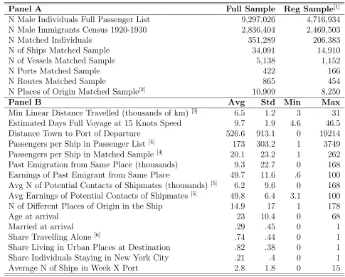
Summary Statistics Table 1 presents some summary statistics of the data. Panel A reports aggregated information on the number of individuals, ships and places of origin for different sub-samples and data sources. The first column (full sample) includes individuals
25The algorithm generates the following information: latitude and longitude of the place, name
iden-tified by the Google Places Api and the south-west/north-east coordinates of the smallest rectangle containing the place. A 20% of the records have missing information on the place of origin and a 15% of the observations are geocoded with a precision above the locality level (e.g. province).
26All these variables are created by the Minnesota Population Center and are comparable across
individuals and census years (Ruggles et al. 2015).
27Although these variables are not directly comparable with more recent industry or occupation
from any origin and age group. The matching rate, defined as the number of matched individuals with respect to the individuals observed in the Censuses, is 12.4%. Matched individuals are observed in approximately 34,000 different ships, departing from 422 ports and proceeding from 10,900 different places of origin.28 After restricting the sample to
individuals in the age group 14-65 with non-missing information on the place of origin and to ships departing from ports at a minimum distance of 3000 km. from New York, approximately 206,000 individuals from 15,000 ships, 170 ports and 8,200 places of origin remain in the sample.
Panel B reports basic statistics on individual and ship characteristics. Ships in the regression sample travelled an average distance of 6,500 kilometers (whole route). This distance would take about 10 days at 15 nautical knots, the average speed for steamers in that period. In the full passenger list data, an average ship transported 173 male passengers in the age group 14-65 (excluding those boarding at less than 3000 km from New York). Ship size is consistent with the findings in Bandiera et al. (2013) for the same period.29The average number of passengers per ship observed in the matched sample
was about 20. Ships were very diverse in terms of places of origin: an average ship transported individuals from 15 different towns of origin (in the matched sample). A large proportion of passengers were single and travelled without any relative. At destination, most immigrants settled in urban places and 21% were observed living in New York in the next Census after their arrival.
4
Empirical Setting
In this section, I explain the empirical strategy to estimate the effects of brief social interactions, and then justify it with a set of balancing tests. Establishing this causal effect is not an easy task. In addition to considering the exogenous allocation of individuals across ships, I need to consider the possibility that shipmates’ characteristics can affect earnings through channels that do not require social interaction. I postpone the discussion of these confounding effects to Section 6, were I provide additional evidence on the social interaction mechanism.
28Table 1 indicates that 15% of places of origin are geographical units above the locality level (e.g.
province). As a robustness check, in Appendix B I re-estimate the main results excluding these geograph-ical units
29Bandiera et al. (2013) find that for the period 1892-1924, the average number of passengers per
Defining Brief Social Interactions The first step in the analysis requires defining the set of individuals who met for the first time during the voyage. For every individual, I identify this set byexcluding any shipmate such that 1) shares the same town of origin or 2) has a similar surname, defined as aJaro-Winkler distance below 0.1.30’31 Along the
paper, I will refer to them as the set ofunrelated shipmates. In Section 5, I perform a set of exercises to rule out the chance that effects are driven by a weak definition of unrelated shipmates.
Connections on Arrival An important variable that I use below is the quality of po-tential contacts that immigrants had in the US. This is a key variable in the empirical strategy as I will proxy the quality of shipmates based on this dimension. Following a number of influential papers (e.g. Wegge, 1998; Munshi, 2004; McKenzie & Rapoport, 2007, 2010) I define the set of potential contacts at destination, as those individuals who emigrated in the past from the same place of origin. There are two additional rea-sons to use the community of origin as the relevant unit to define the social network at destination. First, there is a strong consensus among historians on the importance of settled immigrants in triggering chain migration and supporting new arrivals from the same community (Daniels, 2002). Second, during this period the outcomes of newcom-ers are strongly correlated with the characteristics of settled immigrants from the same community.
To measure the quality of contacts on destination, I focus on two variables:32
1) The average earnings score of settled immigrants from the same town of origin.
2) The number of individuals from the same town who emigrated to the US in the past.33
30The Jaro-Winkler distance (Winkler, 1999) measures the similarity between two words based on the
number and position of common characters.
31In addition to these conditions, I use the smallest rectangular area containing the place of origin
to exclude any shipmate with area overlapping above 50%. This additional condition assures that no shipmate is considered “unrelated” due to a poor geocoding information (e.g. a shipmate with the same province of origin but without information on the exact town of origin). In Section 5, I show that the main results are robust to more strict conditions (e.g. excluding close towns)
32As a robustness check, in Section 5, I re-estimate the main results using alternative definitions of
connections on arrival.
33The earnings of settled immigrants are calculated only for towns observed in the matched sample
The first variable proxies the economic status of potential contacts, based on the notion that wealthier connections can provide information or referrals on better jobs. The second variable proxies the size of the network at destination.34
Formally, I define xc(k),t(k) as the earning score for an individual k from town
c(k) and who travelled in period t(k). This notation emphasizes the fact that each individual in the data is associated to a unique town of origin and emigration period. The average earnings of potential connections on land for individual j is defined as
Xc(j),t(j) = Prt−(k1)=1xc(k),r(k)/Nc(j),t(j) with Nc(j),t(j) being the number of individuals from
townc(j) who emigrated before periodt(j) and are observed in the census.35 The number
of potential contacts upon arrival for individual j, defined as Zc(j),t(j), can be measured
as the size of emigration flows from town c(j) to the US before period t(j). Note that
Zc(j),t(j) is measured using the whole passenger list but Xc(j),t(j) and Nc(j),t(j) are
calcu-lated using the matched sample only. This underlines the complementarity of the two measures. Table 1 Panel B, reports summary statistics about these variables. Earnings of potential contacts are measured in the scale of 0 to 100 and the average in the sample is 49.7. The average number of potential contacts of an individual is 9,300.
Figure 4 illustrates the relevance of previous definitions. Each panel of the figure displays the coefficients of the following regressions between individual outcomes and the quintiles of his potential contacts’ characteristics, conditional on ship and predetermined individual characteristics:
Yi =
5
X
q=1
βqContactsCharqi + σs(i)+ αIi+ ǫi (1)
where Yi is an outcome of individual i (measured at the next Census after arrival),
ContactsChariq is a dummy for the quintile q of some characteristic of the potential con-tacts of the individual (e.g. the number of individual’s concon-tactsZc(i),t(i)). Each regression
controls for ship fixed effectsσs(i) and a set of predetermined individual characteristicsIi.
Panel A shows the correlation between individual earnings and the average earnings (and number) of settled immigrants from the same town of origin. Panels B to D shows that the location of individuals and the sector of occupation are strongly correlated with those of previous emigrants from the same place. Thus, even if newcomers never interact with settled immigrants, we can think that at the moment of the trip, the previous definitions are predetermined predictors of immigrants’ economic success.
34Previous studies have measured the migrant network size in different ways. For instance, Munshi
(2003) measures it as the share of immigrants from the home community while Beaman (2012) uses the number of individuals from the same country living in a given city.
35Note that earnings scores of individuals arrived in different years are usually observed in the same
Identification Strategy In order to identify the effects of brief social interactions, I rely on the assumption that, conditional on their towns of origin, individuals departing from the same port and in the same week, were plausibly exogenously assigned to ships. The plausibility of this assumption is empirically validated later in this section. The intuition behind the identification strategy can be illustrated with the following example: Assume that an individual with residence in Benevento (Italy) has decided to emigrate from the port of Naples (the closest to his town). Naturally, individuals departing in different years or seasons, may face different conditions at departure or arrival. Consequently, shipmates’ characteristics can be correlated with unobserved determinants of the individual’s earnings at destination. Consider, however, all the ships departing from Naples within a relatively narrow time horizon (e.g. a week). The identification strategy relies on the assumption that the individual assignment is uncorrelated with the characteristics of the unrelated shipmates boarding the same ship.36
A number of historical facts support this assumption. First, the selection among passengers of different income took place mainly within ships, as every vessel had different classes and service upgrades. For instance, wealthy individuals usually travelled in first or cabin classes. Second, during a short window of time, the fares for lower class categories (e.g. third class or steerage) were remarkably similar across shipping lines for a given route.37 The vast majority of immigrants travelled in steerage class. Third, delays due
to paperwork or unexpected changes announced by the shipping company were common. Finally, passengers bought their tickets days or weeks in advance, without being able to anticipate the characteristics of their potential shipmates. Naturally, the exogeneity claim must be validated in the data, and in this section I discuss a number of empirical exercises that support this assumption.
A potential concern is that some vessel characteristics (for instance, their external look or capacity) can influence the individual decision, creating some endogenous sorting of passengers. In Section 5, I show that results are robust to the inclusion of a large set of ship characteristics and even of vessel fixed effects. Moreover, as shown below in this section, ship characteristics are strongly balanced with respect to the average shipmates’ quality.
The exogenous allocation across ships, creates quasi-experimental variation in the
36In Section 5, I explore two alternative identification strategies based on the variation created by
repeated voyages of the same vessel and by individuals boarding at different ports during the same trip.
37For instance, Hopkings (1910) reports that in 1909, all the steamers covering the Mediterranean
pool of (unrelated) shipmates of each passenger. This implies that similar individuals can be exposed to a pool of shipmates with different quality of connections on land. An advantage of this strategy follows from the fact that the characteristics of contacts upon arrival are predetermined variables at the moment of the trip, thus not affected by any shock occurring after departure.
Estimating Equation The baseline estimating equation is:
Yi =β1X¯i + β2Z¯i + θp(i)×λw(i) + δc(i)×πt(i)+ ǫi (2)
where Yi is a labor market outcome for immigrant i in the US. Consistently with
the earlier discussion, I control for the interaction betweenθp(i)(a fixed effect for the port
of departure) andλw(i) (the fixed effect for the week of arrival).38
The main variables of interest, ¯Xi and ¯Zi, measure the quality of the connections of
i’s shipmates. The first variable is the average earnings score of the potential connections on land among i’s shipmates. The second measure, is the average number of potential contacts amongi’s shipmates. As discussed in Section 3, potential connections on land for individualj are defined as the set of emigrants from the same town of origin. Formally, if u(i, s) is the subset of passengers travelling in ships and unrelated to i, I define ¯Xi =
P
j∈u(s,i)Xc(j),t(j)/nu(s,i)withnu(s,i)being the number of unrelated shipmates for individual
i. Similarly, I define ¯Zi =
P
j∈u(s,i)Zc(j),t(j)/nu(s,i).39 As defined before in this Section, for
a given individual j, Xc(j),t(j) is the average earnings in the US among individuals from
townc(j) who emigrated before period t(j) and Zc(j),t(j) is the total emigration flow from
townc(j) to the US before periodt(j).
The baseline specification also controls for the interaction between δc(i) (a fixed
effect for the town of origin of immigrant i) and πt(i) (a fixed effect for the semester
of arrival). The inclusion of this interaction serves two purposes. First, it controls for
38Note that I do not observe the week of departure, however, conditional on the port of departure,
this is similar to control for the week of departure. Moreover, the route of the ship accounts for almost all the variation in voyage duration. In Section 5, I present evidence that results are robust to the inclusion of the route fixed effects.
39Some technical aspects involved in the calculation are worth mentioning: (a) Note that both variables
unobserved time-variant characteristics that could result in individuals from specific towns boarding certain ships with higher probability. This would be the case, for instance, if agencies sold tickets for different ships with varying intensity across regions of the country. Second, given that potential connections on land are defined at the town of origin level, it absorbs any characteristic of individual’s own contacts. As discussed in Caeyers & Fafchamps (2017), this strategy eliminates any negative exclusion bias (Guryan et al., 2009) introduced by the fact that i’s connections are excluded in the calculation of ¯Xi
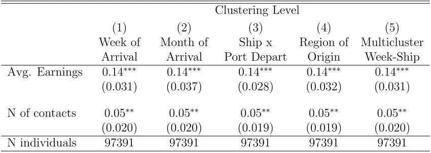
and ¯Zi.40 All regressions cluster standard errors at the week of arrival level. In Appendix
Table A2, I show that baseline estimates are robust to alternative clustering choices.
Balancing Tests and Evidence of Exogenous Sorting This subsection discusses a number of tests supporting the identifying assumption outlined before. This is critical to establish a causal interpretation of the effects of shipmates’ characteristics on future labor outcomes.
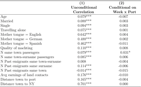
The first test consists of studying the correlation between the predetermined vari-ables of an individual and those of his unrelated shipmates. The exogeneity claim requires that this correlation must be zero after conditioning on the interaction between the port of departure and the week of arrival. Therefore, for every individual in the matched sample, I calculate the average characteristics of his unrelated shipmates. In order to avoid the negative mechanical bias of leave-one-out correlations, I follow Baker et al. (2008) and sample one individual per ship when performing these calculations. Column 1 of Table 2 reports the unconditional correlations and Column 2 conditions on Port of Departure X Week of Arrival.41 Results indicate that the unconditional correlations are high and
significant but all of them become low and insignificant (at 5% level) after controlling for Port of Departure X Week of Arrival.42
The second set of tests is given by standard balance regressions. This consists of OLS regressions of a number of predetermined passenger and ship characteristics on the two main variables of interest, ¯Xi and ¯Zi. The results in Figure 5, where I label
each row in the left axis by the dependent variable, plot the estimated 95% confidence intervals of the regression. Panel A plots the confidence intervals for the average earnings
40I define π
t(i) at semester level due to the relatively small size of most towns of origin. For instance,
I observe very few week-port cells with more than one individual from the same town boarding different ships. In Section 5, I show that results are robust to controlling for the interaction between town of origin and the month of arrival.
41A number of predetermined characteristics in the test vary at the town of origin level, for this reason,
I do not control for the town of origin fixed effect, but on a larger geographical level (e.g. provinces in the case of italy). Note however, that this imposes a more demanding condition for balance.
42Significance levels are bootstrapped by repeating 500 times the procedure of sampling one individual
of unrelated shipmates’ contacts on land. Similarly, Panel B corresponds to the average number of shipmates’ potential connections on land. To illustrate the importance of the baseline controls, I report the estimates with and without the Port of Departure X Week controls.43 To ease interpretation, all variables in the regressions are standardized.
I find that shipmates’ characteristics are (unconditionally) correlated with individ-ual and ship characteristics: the estimates are statistically significant for most dependent variables. The introduction of the baseline controls, however, greatly decreases the esti-mates which become extremely small in magnitude. For any left hand side variable, the coefficients imply that one standard deviation in either the number or the earnings of unrelated shipmates’ contacts on land, has an effect lower than 0.05 standard deviations. Indeed, after controlling for Port X Week, only two of the 32 displayed coefficients are statistically different from zero at the 5% level.44
Overall, I interpret the results of this subsection as supporting the exogeneity of the variation of shipmates’ characteristics among unrelated individuals departing from the same port during a given week. Consequently with these findings, In Section 5 I provide additional support for the identification assumption, by showing that the results are robust to the inclusion of a large set of additional controls.
Census-Ships Data Matching and Non-Random Sampling A potential concern in the study is that the matching process creates a non-random sample of the ships. A number of additional findings suggest that, conditional on baseline controls, matching is not systematically correlated with individual or ship characteristics.
First, note that the dependent variable in the last row of Figure 5 is the (stan-dardized) share of matched passengers within the ship. Conditional on the Week X Port controls, the correlation is extremely low in magnitude: One standard deviation increase in ¯Xior ¯Zi, changes the matching rate in less than 0.02 standard deviations. Figure 6
fur-ther explores this idea and estimates the balance equation for quintiles of the shipmates’ contacts characteristics.
Second, I estimate the correlation between the ship matching rate and a set of individual predetermined characteristics conditional on similar controls than those in the balance regressions. Figure 7 plots this regression. Estimated coefficients are insignificant
43Following the discussion in footnote 41, regressions include fixed effects for large administrative
units. Additionally, in order to eliminate any potential downward exclusion bias (Guryan et al., 2009), I control for the earnings and number of passenger’s own potential connections. Appendix Figure A3 displays similar balancing tests using the same controls and sample used in the baseline specification (variables defined at town of origin level are then excluded)
44Since the right hand side variables can be correlated with each other, Appendix Figure A2 displays
for 12 out of 13 variables and low in magnitude in every case. Along with the balance tests, this evidence suggests that conditional on baseline controls, the matching algorithm does not correlate with individual outcomes. This is not surprising as surname characteristics are the main determinants of the matching rate, and within the Week X Port cell, they are not systematically different.
Finally, I use the full Passenger List data to study whether the probability of being matched correlates with ships characteristics. I regress a dummy variable indicating if the passenger was matched to Census on the full set of Ship fixed effects. Table 3 reports the F-statistic for the joint significance test of Ship fixed effects. Column (1) shows that without further controls, Ship fixed effects have significant predictive power on the matching rate. However, as shown in Column (2), after including the Week X Port fixed controls, Ship fixed effects are jointly insignificant.45
These findings also highlight an advantage of the empirical strategy: Even if match-ing is non-random for the whole sample (e.g. because some nationalities are easier to match), narrowing the variation to the Week X Port of Departure level eliminates any significant difference in matching rates across ships or individuals.
5
Baseline Results
This section describes and interprets the baseline results of the paper. I also show that the effects of travelling with better connected shipmates persisted for years after the arrival. I then discuss a number of robustness tests aimed to provide additional support for the identification assumption. Finally, I discuss the robustness of results to alternative specifications and clustering of standard errors.
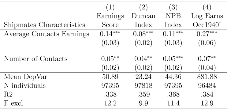
Baseline Estimates Table 4 reports estimates of Equation (2) for different measures of earnings and job quality. Column (1) indicates that both dimensions of shipmates’ contacts quality have a positive and significant effect on individual earnings score. Expo-sure to shipmates with connections employed in jobs one percentile higher in the earnings distribution, increases individual earning score in 0.14 points. Similarly, every thou-sand additional (average) connections among shipmates increases earnings score by 0.05.
45A different concern is related to the partial observability of the relevant network structure. Under
Columns (2) to (3) reports the results for the alternative measures of job quality dis-cussed in Section 3. Estimates indicate effects of a similar magnitude.46 Although these
variables are correlated with the earning score, they measure different aspects of job qual-ity. Understanding the size of effects based on Earnings Score is not straightforward as the earning distribution is typically left-skewed. In order to ease the interpretation of my findings, I also report the estimates of Equation (2) when the dependent variable is the logarithm of the earnings derived from the 1940 Census.47 Findings in Column (4)
mean that an upward shift of 10 percentiles along the income distribution of shipmates’ connections, increases individual earnings by 2,7%. Every thousand additional (average) connections among unrelated shipmates, increases earnings by 0.7%.48
Equation (2) can hide some non-linear relationship between individual earnings and shipmates’ connections quality. A potential concern is that results are driven by few ships with outlier characteristics. Figure 8 displays non-parametric evidence that the effects are increasing in the quintiles of the variables of interest. In the case of shipmates’ connections earnings, effects are monotonically increasing and statistically significant for quintiles 3 to 5. Travelling in a ship in the highest quintile, increases individual earnings score in 1.8 points with respect to the lowest quintile (an effect of 4% according to the regression with log-earnings in panel B). In the case of the number of connections, the effects are weakly increasing but only significant for the highest quintile. Travelling in a ship among the highest quintile of this variable, increases individual earnings score by 1 point with respect to the lowest quintile (an increase of 2% based on the regression with log-earnings displayed in panel B). It is useful to compare these figures with the estimated correlations between earnings and the characteristics of individual’s own connections in the US (Panel A of Figure 4). Although the later is not necessarily causal, it is a useful benchmark for interpreting the magnitude of the effects. Not surprisingly, the effects of shipmates’ connections on earnings are lower than the correlation with respect to the own contacts’ characteristics. For instance, relative to the lowest quintile, the effect of travelling with shipmates in the highest quintile of contacts’ earnings is three to four times lower than the effects of having connections in the highest quintile of earnings.
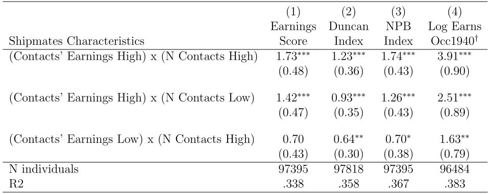
Appendix Table A3 explores the interaction between the two measures of quality
46The Duncan Socioeconomic Index, reflects the social perception of the “prestige” associated to an
occupation. The Nam-Power-Boyd index captures differences in the education-earning composition of different occupations. Both variables have the same scale than the earnings score (0 to 100).
47The construction of this variable is described in Section 3.
48Appendix Table A1 reports the results for two additional variables based on the 1950 Census. The
of shipmates’ connections. The estimated coefficients correspond to an OLS regression (analogous to Equation (2)) where the explanatory variables are the interactions between two sets of dummies indicating whether the number of shipmates’ connections or their average earnings are above/below the median of its distribution. Both measures of con-nections’ quality are relevant. Starting from a situation where shipmates have low-quality connections in terms of both earnings and number, an increase in either dimension has a positive impact on earnings. Table A3 also suggests that the earnings of shipmates’ connections is relatively more important than the number of shipmates’ connections.
The baseline effects display some heterogeneity at geographical level. Appendix Figure A5 plots the estimates of Equation (2) where the shipmates contacts’ earnings variable is interacted with dummies for the country of origin of the individual. The map shows the relative size of the effects for Europe. Among countries with more emigrants in the data, effects are stronger for Ireland, Poland and Greece. Naturally, other factors correlated with the country of origin can drive the heterogeneous effect. For instance, the estimated effect for Italians is significant but below the median for Europe. This could be partially explained by the fact that Italians from distant regions typically spoke different languages. Unsurprisingly, the potential benefits of social interactions might depend on the ability to communicate with those well connected shipmates.
Persistence of the Effects Due to the low number of arrivals between 1914 and 1919, most immigrants in the data are observed many years after arrival (7.5 years on aver-age). This suggests that effects of social interactions with unrelated shipmates is highly persistent. Figure 9 explores this idea in more detail and displays the estimates of the baseline equation where the right hand side variables are interacted with dummies for each year since arrival. Although this disaggregation can confound other characteristics correlated with the time since arrival, the figure suggest that effects are not only driven by recent migration. Moreover, estimated effects are statistically significant even 10 years after arrival.49
49There are two main confounders for this heterogeneous effect. First, earlier arrivals are older when
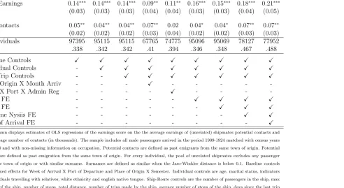
Additional Controls In this subsection I show that results are robust to the inclusion of a large number of additional controls. This evidence is important to rule out some potential threats to the validity of the identification strategy. Table 5 summarizes all these findings. Columns (2) and (3) show that estimates are robust to the inclusion of a set of individual characteristics (age, race, marital status, language, and an indicator for the individual travelling with some relative) and a set of characteristics of the ship and the route (e.g. ship capacity, number of passengers, distance travelled, number of stops, share of male passengers, etc.). Robustness to these controls is consistent with the assumption that, conditional on baseline controls, the pool of shipmates is not correlated with individual or ship characteristics. In a more general way, I want to rule out that individuals select into ships due to unobservable characteristics of the ship. This would be the case if for instance, more educated individuals (which potentially correlates with their connections quality) select into ships with higher capacity or higher speed. Such sit-uation would confound the effect of better connected shipmates with individual’s different characteristics. Column (6) shows that effects are similar after controlling for vessel fixed effects and this finding is inconsistent with such interpretation.
Note that the baseline specification (Equation (2)) absorbs any shock at the Town of Origin X Semester level. Although this is an already narrow time-space grid, some concerns may arise regarding the relevant time horizon in which local shocks can affect passengers’ predetermined characteristics.50 Column (4) extends the baseline specification
to a shorter window of time by controlling for the interaction between fixed effects of the town of origin and the month-year of arrival. Since most towns are relatively small, there are fewer cells with multiple individuals from the same town boarding different ships within the same month. Despite of the lower number of observations, results remain statistically significant with coefficients of similar magnitudes. Column (5) narrows the time horizon to the week level but uses a larger spatial aggregation grid (administrative units above the locality level, e.g. provinces in the case of Italy). In this case, results are similar for the earnings of shipmates’ contacts and non-significant for the number of connections on land, although standard errors are also larger due to the introduction of a large number of fixed effects.
As discussed in Section 4, it is possible that ships departing from the same port during the same week, followed a different route. Although the vessel fixed effect controls for most of this variation, some vessels could have covered different routes over time. Column (7) shows that baseline results are robust to the inclusion of fixed effects for each
50For instance, it could be the case if a local shock greatly changes the quality of individual’s own
route identified in the data. This rule out that results are driven by some correlation among shipmates’ characteristics created by individuals selecting across ships based on the travelled route.51
Finally, Columns (8) and (9) aim to control for a narrow set of individual char-acteristics and labor market conditions upon arrival. Column (8) includes fixed effects for the NYSIIS phonetic coding of surnames (Atack & Bateman, 1992) which accounts for approximately 8000 groups of surnames.52 Column (9) includes fixed effects for the
date of arrival. Despite of a lower number of observations, estimates are robust to the inclusion of the additional controls. These findings have a number of implications. First, surnames embeds some important unobserved characteristics of individuals. Thus, find-ings are consistent with the claim that conditional on baseline controls, passengers do not select into ships according to individual characteristics that correlate with earnings. Second, surname is the most critical variable when matching between Passenger Lists and Censuses. Some surnames are more difficult to match either because they are too frequent, or because they are more likely to be misspelled when transcribed. Therefore, results in Column (8) are inconsistent with a non-random matching across ships driving the results. Lastly, results in Column (9) rule out that some correlation between ship-mates’ characteristics and daily conditions upon arrival explains my findings. This would be the case if for instance, the arrival of passengers from certain towns triggered some events like a higher demand for train tickets to some destinations or a lower availability of temporary accommodation in New York City.
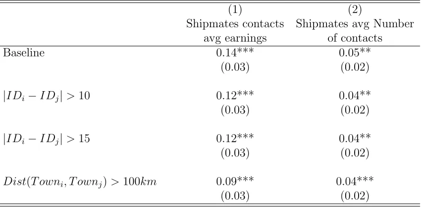
Narrowing the Definition of Unrelated Shipmates One potential concern when establishing a causal interpretation of Equation (2) is the possibility that shipmates from different places of origin are already connected before travelling. Although this is an unlikely event for the vast majority of passengers, I restrict in two ways the pool of shipmates assumed to be unrelated. First, I use the fact that travelling together (or buying the ticket from the same agent) typically implied nearby manifest line numbers. Appendix Figure A4 shows an example of this situation where members of the same family follow the same order.53 In Table 6, I report the estimates of the baseline equation but 51This is not surprising given that the ports concentrating most of the departures in this period are
usually covered by few routes, and in many cases by a unique route.
52Including surname fixed effects is problematic for two reasons. First, the large variety of different
surnames would absorb most of the variation at individual level. Second, a non-negligible part of the variation in surnames can be due to transcription errors or typos.
53Although families are almost always in the same block within the manifest, this practice was not
for every individual, I restrict the set of his unrelated shipmates by imposing a minimum distance in their ID numbers (which follows the same order than manifest line numbers). The first two rows of the table exclude any shipmate with a difference in ID numbers lower than 10 and 15 respectively. The second way in which I restrict this set is by excluding passengers with towns of residence located at less than 100 kilometers from each other. The last row of Table 6 displays the baseline results after imposing both sets of restrictions (Minimum ID number difference and minimum distance). Point estimates are somewhat lower for the earnings of shipmates’ contacts (but they remain statistically significant at 1%) and they are similar for the number of shipmates’ connections. Note that either restriction can introduce some attenuation bias if true unrelated shipmates are excluded.54 Moreover, due to language constraints and social preferences, interaction
with unrelated individuals can be more likely to occur among those from closer towns.
Alternative Definition of Connections on Arrival As discussed in Section 4, defin-ing potential contacts in the US at the town of origin level is in line with a number of previous studies. However, in the setting of this paper, it is possible to think that nar-rower definitions of connections are also relevant (for instance, relatives who emigrated in the past). In Appendix Table A5, I re-estimate the baseline specification using two alter-native definitions of potential connections upon arrival to the US. First, in Column (2) I consider individuals with similar surname (based on the NYSIIS coding) who previously emigrated from the same province or large administrative unit. Second, I consider past emigrants from the same town of origin who share a similar surname (Column (3)). For small places, the second definition captures to a large extent, relatives who emigrated in the past. In order to ease the comparison across definitions, I standardize all the right hand side variables. Column (1) corresponds to the baseline definition.55 Alternative
definitions result in estimated effects of similar magnitude, and in both cases, higher than the baseline results. Higher estimates can be due to a number of reasons. First, unique surnames are not included in the pool of unrelated individuals when computing earnings of shipmates contacts. Second, given a narrower definition, within ship variation in ship-mates’ characteristics is also larger. Finally, connections with settled emigrants of similar surname can be the main source of information and support upon arrival, or just better predictors of economic success for immigrants.
54See footnote45
55Narrowing the definitions for potential contacts significantly reduce the number of observations and
Alternative Identification Strategies I explore two additional sources of variation in the characteristics of shipmates. The first strategy exploits the fact that many vessels traveled from the same port repeatedly during the year. Therefore, I only compare pas-sengers travelling in the same vessel within the same semester. Column (1) in Appendix Table A6 estimates the following equation:
Yi =β1X¯i + β2Z¯i + ψv(i)×θp(i)×λy(i) + δc(i)×πt(i) + ηr(i)×πt(i) + ǫi (3)
where ψv(i) is a vessel fixed effect, ηr(i) is a route fixed effect and the rest of variables
are defined identically to Equation (2). Estimates for this specification are displayed in Column (1). Point estimates are highly significant for the case of earnings of shipmates’ contacts and the magnitude is approximately 40% lower than the baseline effects. These results provide additional evidence that baseline effects are not driven by passengers sorting across vessels.
The second alternative variation follows from the fact that some ships stopped at different ports before arriving New York. In this case, I exploit the variation in shipmates’ characteristics created by passengers from different ports. A potential concern of this specification is that some ports can be very distant from each other reducing the potential interaction between these shipmates. Moreover, in many cases, shipmates boarding at different ports spoke different languages.56 Additionally, the sample size is largely reduced
because either there were no intermediate stops or because only few individuals boarded at a different port. Indeed, I exclude any ship where more than 90% of the passengers boarded in the same port. Column (2) estimates the following equation:57
Yi =β1X¯isp + β2Z¯isp +α1X¯idp + α2Z¯idp + ψv(i) + δc(i)×πt(i) + ηr(i)×πt(i) + ǫi (4)
where ¯Xisp, ¯Z sp i , ¯X
sp
i and ¯Z sp
i are defined similarly to Equation (2) but I distinguish
between the characteristics of passengers boarding in the port (superscript sp) and that of those boarding at a different port (superscript dp). Estimates from this equation are displayed in Column (2). Point estimates are higher for the characteristics of same-port shipmates and only significant for the earnings of shipmates’ contacts. Finally, in Column (3) I only consider individuals who boarded the ship at the first departing port and use
56This was true not only for ships stopping at different countries. For instance, italians boarding at
different ports typically spoke different languages/dialects and fluent communication among them was very unlikely.
57Note that I don’t include the interaction between port of departure and the time dimension in order
the variation created by shipmates boarding at subsequent ports. Remarkably, point estimates for the earnings of shipmates’ contacts are similar to those in Column (2).58
6
Mechanism: Establishing a Social Interaction
In-terpretation
The findings in the previous Section, show a causal link between the short run exposure to a pool of better connected individuals and future performance in the labor market. However, this reduced form result is compatible with a number of mechanisms that do not necessary require social interaction among unrelated shipmates. In this Section, I provide evidence supporting the social interaction interpretation as the most plausible one.
I start by showing, that the effect is stronger for passengers with fewer connections and that results are driven, to a larger extent, by shipmates speaking the same language (a natural mediator of social interaction). Then, I show that the sector of employment and place of residence of shipmates’ contacts have predictive power on the occupational and residential outcomes of the individual. Finally, as a reassuring exercise, I show that conditional on arriving in the same week and from the same port, the correlation in labor and residential outcomes is stronger among shipmates.
Heterogenous Effects As described in Section 3, this was a period of high-stakes decisions for most immigrants. Consequently, the effects of brief social interaction are expected to be higher for individuals with poor connections and no access to relevant information. Table 7 displays estimations of the baseline regression where each measure of shipmates’ connections is interacted with dummies indicating how well connected is the individual himself. Column (1) explores the quality of connections on board, that is, whether the passenger is travelling alone or with relatives.59 Individuals travelling
alone are more benefited by travelling with higher quality shipmates. Column (2), shows that individuals with poor connections on land60 are more affected by their shipmates’
contacts characteristics. Finally, Column (3) shows that effects are stronger for individuals travelling aloneand with poor connections on land.
58This also illustrates that my identification strategy is robust to exclusion bias (see Angrist, 2014). 59In order to avoid confounding the effect with the surname prevalence, I include surname NYSIIS
code fixed effects. This explains why, consistent with Table 4, the average effect is higher compared to the baseline.
60An individual is defined as low connected when the median earnings and the median number of past