An analysis of the user occupational class through Twitter content

An analysis of the user occupational class through Twitter content

Daniel Preot¸iuc-Pietro1_{, Vasileios Lampos}2 _{and Nikolaos Aletras}2

1_{Computer & Information Science, University of Pennsylvania} 2_{Department of Computer Science, University College London} danielpr@sas.upenn.edu, {v.lampos,n.aletras}@ucl.ac.uk

Abstract

Social media content can be used as a complementary source to the traditional methods for extracting and studying col-lective social attributes. This study focuses on the prediction of the occupational class for a public user profile. Our analysis is conducted on a new annotated corpus of Twitter users, their respective job titles, posted textual content and platform-related attributes. We frame our task as classifi-cation using latent feature representations such as word clusters and embeddings. The employed linear and, especially, non-linear methods can predict a user’s occupational class with strong accuracy for the coars-est level of a standard occupation taxon-omy which includes nine classes. Com-bined with a qualitative assessment, the derived results confirm the feasibility of our approach in inferring a new user at-tribute that can be embedded in a multitude of downstream applications.

1 Introduction

The growth of online social networks provides the opportunity to analyse user text in a broader context (Tumasjan et al., 2010; Bollen et al., 2011; Lam-pos and Cristianini, 2012). This includes the social network (Sadilek et al., 2012), spatio-temporal in-formation (Lampos and Cristianini, 2010) and per-sonal attributes (Al Zamal et al., 2012). Previous research has analysed language differences in user attributes like location (Cheng et al., 2010), gender (Burger et al., 2011), impact (Lampos et al., 2014) and age (Rao et al., 2010), showing that language use is influenced by them. Therefore, user text al-lows us to infer these properties. Thisuser profiling is important not only for sociolinguistic studies, but also for other applications: recommender systems

to provide targeted advertising, analysts who study different opinions in each social class or integra-tion in text regression tasks such as voting intenintegra-tion (Lampos et al., 2013).

Social status reflected through a person’s occu-pation is a factor which influences language use (Bernstein, 1960; Bernstein, 2003; Labov, 2006). Therefore, our hypothesis is that language use in social media can be indicative of a user’s occu-pational class. For example, executives may write more frequently about business or financial news, while people in manufacturing positions could re-fer more to their personal interests and less to job related activities. Similarly, we expect some cate-gories of people, like those working in sales and customer services, to be more social or to use more informal language.

Focusing on the microblogging platform of Twit-ter, we explore our hypothesis by studying the task of predicting a user’s occupational class given platform-related attributes and generated content, i.e. tweets. That has direct applicability in a broad range of areas from sociological studies, which analyse the behaviour of different occupations, to recruiting companies that target people for new job opportunities. For this study, we created a publicly available data set of users, including their profile information and historical text content as well as a label to an occupational class from the “Stan-dard Occupational Classification” taxonomy (see Section 2).

We frame our task as classification, aiming to identify the most likely job class for a given user based on profile and a variety of textual features: general word embeddings and clusters (or ‘topics’). Both linear and non-linear classification methods are applied with a focus on those that can assist in-terpretation and offer qualitative insights. We find that text features, especially word clusters, lead to good predictive performance. Accuracy for our best model is well above 50% for 9-way

cation, outperforming competitive methods. The best results are obtained using the Bayesian non-parametric framework of Gaussian Processes (Ras-mussen and Williams, 2006), which also accom-modates feature interpretation via the Automatic Relevance Determination. This allows us to get in-sight into differences in language use across job classes and, finally, assess our original hypothesis about the thematic divergence across them.

2 Standard Occupational Classification

To enable the user occupation study, we adopt a standardised job classification taxonomy for map-ping Twitter users to occupations. The Standard Oc-cupational Classification (SOC)1_{is a UK}

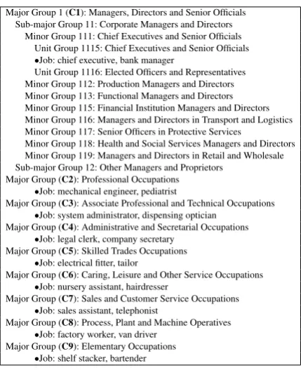
govern-ment system developed by the Office of National Statistics for classifying occupations. Jobs are cate-gorised hierarchically based on skill requirements and content. The SOC scheme includes nine major groups coded with a digit from 1 to 9. Each ma-jor group is divided into sub-mama-jor groups coded with 2 digits, where the first digit indicates the ma-jor group. Each sub-mama-jor group is further divided into minor groups coded with 3 digits and finally, minor groups are divided into unit groups, coded with 4 digits. The unit groups are the leaves of the hierarchy and represent specific jobs related to the group.

Table 1 shows a part of the SOC hierarchy. In to-tal, there are 9 major groups, 25 sub-major groups, 90 minor groups and 369 unit groups. Although other hierarchies exist, we use the SOC because it has been published recently (in 2010), includes newly introduced jobs, has a balanced hierarchy and offers a wide variety of job titles that were crucial in our data set creation.

3 Data

To the best of our knowledge there are no pub-licly available data sets suitable for the task we aim to investigate. Thus, we have created a new one consisting of Twitter users mapped to their oc-cupation, together with their profile information and historical tweets. We use the account’s profile information to capture users with self-disclosed occupations. The potential self-selection bias is ac-knowledged, but filtering content via self disclosure

1_{http://www.ons.gov.uk/ons/}

guide-method/classifications/ current-standard-classifications/ soc2010/index.html; accessed on 24/02/2015.

Major Group 1 (C1): Managers, Directors and Senior Officials Sub-major Group 11: Corporate Managers and Directors

Minor Group 111: Chief Executives and Senior Officials Unit Group 1115: Chief Executives and Senior Officials

•Job: chief executive, bank manager

Unit Group 1116: Elected Officers and Representatives Minor Group 112: Production Managers and Directors Minor Group 113: Functional Managers and Directors Minor Group 115: Financial Institution Managers and Directors Minor Group 116: Managers and Directors in Transport and Logistics Minor Group 117: Senior Officers in Protective Services

Minor Group 118: Health and Social Services Managers and Directors Minor Group 119: Managers and Directors in Retail and Wholesale Sub-major Group 12: Other Managers and Proprietors

Major Group (C2): Professional Occupations

•Job: mechanical engineer, pediatrist

Major Group (C3): Associate Professional and Technical Occupations

•Job: system administrator, dispensing optician Major Group (C4): Administrative and Secretarial Occupations

•Job: legal clerk, company secretary Major Group (C5): Skilled Trades Occupations

•Job: electrical fitter, tailor

Major Group (C6): Caring, Leisure and Other Service Occupations

•Job: nursery assistant, hairdresser

Major Group (C7): Sales and Customer Service Occupations

•Job: sales assistant, telephonist

Major Group (C8): Process, Plant and Machine Operatives

•Job: factory worker, van driver Major Group (C9): Elementary Occupations

•Job: shelf stacker, bartender

Table 1: Subset of the SOC classification hierarchy.

is widespread when extracting large-scale data for user attribute inference (Pennacchiotti and Popescu, 2011; Coppersmith et al., 2014).

Similarly to Hecht et al. (2011), we first assess the proportion of Twitter accounts with a clear men-tion to their occupamen-tion by annotating the user de-scription field of a random set of 500 users. There were chosen from the random 1% sample, having at least 200 tweets in their history and with a majority of English tweets. There, we can identify the fol-lowing categories: no description (12.2%), random information (22%), user information but not occu-pation related (45.8%), and job related information (20%).

per-formed by the authors. We also removed users in multiple categories and or users that have tweeted less than 50 times in their history. Finally, we elim-inated all 3-digit categories that contained less than 45 user accounts after this filtering. This process produced a total number of 5,191 users from 55 mi-nor groups (22 sub-major groups), spread across all nine major SOC groups. The distribution of users across these nine groups is: 9.7%, 34.5%, 20.6%, 3.8%, 16.7%, 6.1%, 1.4%, 4.2%, and 3% (follow-ing the order(follow-ing of Table 1). In our data set the most well represented minor occupational groups are ‘Functional Managers and Directors’ (184 users – code 113), ‘Therapy Professionals’ (159 users –

code 222) and ‘Quality and Regulatory Profession-als’ (158 users – code 246), whereas the least rep-resented ones are ‘Textile and Garment Trades’ (45 users – code 541), ‘Elementary Security Occupa-tions’ (46 users – code 924), ‘Elementary Cleaning Occupations’ (47 users – code 923). The mean num-ber of users in the minor classes is equal to 94.4 with a standard deviation of 35.6. For these users, we have collected all their tweets, going as far back as the latest 3,200, and their profile information. The final data set consists of 10,796,836 tweets col-lected around 5 August 2014 and is openly avail-able.2

A separate Twitter data set is used as a reference corpus in order to build the feature representations detailed in Section 4. This data set is an extract from the Twitter Gardenhose stream (a 10% repre-sentative sample of the entire Twitter stream) from 2 January to 28 February 2011. Based on this con-tent, we also build the vocabulary for the text fea-tures, containing the most frequent 71,555 words. We tokenise and filter for English using the Trend-miner preprocessing pipeline (Preot¸iuc-Pietro et al., 2012).

4 Features

In this section, we overview the features used in the occupational class prediction task. They are divided into two types: (1) user level features, (2) textual features.

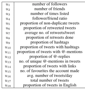
4.1 User Level Features (UserLevel)

The user level features are based on the general user information or aggregated statistics about the tweets. Table 2 introduces the 18 features in this

2_{http://www.sas.upenn.edu/˜danielpr/}

jobs.tar.gz

u1 number of followers

u2 number of friends

u3 number of times listed

u4 follower/friend ratio

u5 proportion of non-duplicate tweets

u6 proportion of retweeted tweets

u7 average no. of retweets/tweet

u8 proportion of retweets done

u9 proportion of hashtags

u10 proportion of tweets with hashtags

u11 proportion of tweets with @-mentions

u12 proportion of @-replies

u13 no. of unique @-mentions in tweets

u14 proportion of tweets with links

u15 no. of favourites the account made

u16 avg. number of tweets/day

u17 total number of tweets

u18 proportion of tweets in English

Table 2: User level attributes for a Twitter user.

category.

4.2 Textual Features

The textual features are derived from the aggre-gated set of user’s tweets. We use our reference corpus to represent each user as a distribution over these features. We ignore the bio field from build-ing textual features to avoid introducbuild-ing biases from our data collection method. While this is a re-striction, our analysis showed that in less than 20% of the cases the information in the bio is directly relevant to the occupation.

4.2.1 SVD Word Embeddings (SVD-E)

We use a more abstract representation of words than simple unigram counts in order to aid inter-pretability of our analysis. We compute a word to word similarity matrix from our reference cor-pus. Normalised Pointwise Mutual Information (NPMI) (Bouma, 2009) is used to compute word to word similarity. NPMI is an information theoretic measure indicating which words co-occur in the same context, where the context is represented by a whole tweet:

NPMI(x, y) =−logP(x, y)·log P(x, y)

P(x)·P(y).

4.2.2 NPMI Clusters (SVD-C)

We use the NPMI matrix described in the previous paragraph to create hard clusters of words. These clusters can be thought as ‘topics’, i.e. words that are semantically similar. From a variety of cluster-ing techniques we choose spectral clustercluster-ing (Shi and Malik, 2000; Ng et al., 2002), a hard-clustering approach which deals well with high-dimensional and non-convex data (von Luxburg, 2007). Spectral clustering is based on applying SVD to the graph Laplacian and aims to perform an optimal graph partitioning on the NPMI similarity matrix. The number of clusters needs to be pre-specified. We use 30, 50, 100 and 200 clusters – numbers were chosen a priori based on previous work (Lampos et al., 2014). The feature representation is the stan-dardised number of words from each cluster.

Although there is a loss of information compared to the original representation, the clusters are very useful in the model analysis step. Embeddings are hard to interpret because each dimension is an ab-stract notion, while the clusters can be interpreted by presenting a list of the most frequent or repre-sentative words. The latter are identified using the following centrality metric:

Cw=

P

x∈cNPMI(w, x)

|c| −1 , (2)

wherecdenotes the cluster andwthe target word.

4.2.3 Neural Embeddings (W2V-E)

Recently, there has been a growing interest in neu-ral language models, where the words are projected into a lower dimensional dense vector space via a hidden layer (Mikolov et al., 2013b). These models showed they can provide a better representation of words compared to traditional language models (Mikolov et al., 2013c) because they capture syntac-tic information rather than just bag-of-context, han-dling non-linear transformations. In this low dimen-sional vector space, words with a small distance are considered semantically similar. We use the skip-gram model with negative sampling (Mikolov et al., 2013a) to learn word embeddings on the Twitter reference corpus. In that case, the skip-gram model is factorising a word-context PMI matrix (Levy and Goldberg, 2014). We use a layer size of 50 and the Gensim implementation.3

3_{http://radimrehurek.com/gensim/}

models/word2vec.html

4.2.4 Neural Clusters (W2V-C)

Similar to the NPMI cluster, we use the neural embeddings in order to obtain clusters of related words, i.e. ‘topics’. We derive a word to word simi-larity matrix using cosine simisimi-larity on the neural embeddings. We apply spectral clustering on this matrix to obtain 30, 50, 100 and 200 word clusters.

5 Classification with Gaussian Processes

In this section, we briefly overview Gaussian Pro-cess (GP) for classification, highlighting our mo-tivation for using this method. GPs formulate a Bayesian non-parametric machine learning frame-work which defines a prior on functions (Ras-mussen and Williams, 2006). The properties of the functions are given by a kernel which models the covariance in the response values as a function of its inputs. Although GPs form a powerful learn-ing tool, they have only recently been used in NLP research (Cohn and Specia, 2013; Preot¸iuc-Pietro and Cohn, 2013) with classification applications limited to (Polajnar et al., 2011).

Formally, GP methods aim to learn a function

f : Rd _{→ R drawn from a GP prior given the}

inputsxxx∈Rd_:

f(xxx)∼ GP(m(xxx), k(xxx,xxx0)), (3)

wherem(·)is the mean function (here0) andk(·,·)

is the covariance kernel. Usually, the Squared Ex-ponential (SE) kernel (a.k.a. RBF or Gaussian) is used to encourage smooth functions. For the multi-dimensional pair of inputs(xxx,xxx0_{), this is:}

kard(xxx,xxx0) =σ2exp

" _d X

i

−(xi−x0i)2

2l2

i

#

, (4)

where li are lengthscale parameters learnt only

using training data by performing gradient as-cent on the type-II marginal likelihood. Intuitively, the lengthscale parameterlicontrols the variation

along theiinput dimension, i.e. a low value makes the output very sensitive to input data, thus mak-ing that input more useful for the prediction. If the lengthscales are learnt separately for each input dimension the kernel is named SE with Automatic Relevance Determination (ARD) (Neal, 1996).

Binary classification using GPs ‘squashes’ the real valued latent functionf(x)output through a logistic function:π(xxx) ,P(y = 1|xxx) = σ(f(xxx))

of the latent variable corresponding to a test case

x∗:

P(f∗|xxx,yyy, x∗) =

Z

P(f∗|xxx, x∗, f)P(f|xxx,yyy)df ,

(5) where P(f|xxx,yyy) = P(yyy|f)P(f|xxx)/P(yyy|xxx) is the posterior over the latent variables. If the likelihood P(yyy|f) is Gaussian, the combination with a GP prior P(f|xxx) gives a posterior GP over functions. In binary classification, the distribution over the latentf∗is combined with the logistic function to

produce the prediction:

¯

π∗=

Z

σ(f∗)P(f∗|xxx,yyy, x∗)df∗. (6)

This results in a non-Gaussian likelihood in the posterior formulation and therefore, exact infer-ence is infeasible for classification models. Multi-ple approximations exist that make the computa-tion tractable (Gibbs and Mackay, 1997; Williams and Barber, 1998; Neal, 1999). In our experiments we opt to use the Expectation Propagation (EP) method (Minka, 2001) which approximates the non-Gaussian joint posterior with a non-Gaussian one. EP offers very good empirical results for many differ-ent likelihoods, although it has no proof of con-vergence. The complexity for the inference step is

O(n3_{). Given that our data set is very large and the} number of features is high, we conduct inference using the fully independent training conditional (FITC) approximation (Snelson and Ghahramani, 2006) with 500 random inducing points. We refer the interested reader to Rasmussen and Williams (2006) for further information on GP classification.

Although we could use multi-class classification methods, in order to provide insight, we perform a separate one-vs-all classification for each class and then determine a label through the occupational class that has the highest likelihood.

6 Experiments

This section presents the experimental results for our task. We first compare the accuracy of our clas-sification methods on held out data using each fea-ture set and conduct a standard error analysis. We then use the interpretability of the ARD length-scales from the GP classifier to further analyse the relevant features.

6.1 Predictive Accuracy

We assign users to one of nine possible classes (see the ‘Major Groups’ on Table 1) using one set of

Feature LR SVM GP

Most frequent class 34.4% 34.4% 34.4%

UserLevel 34.0% 31.5% 34.2%

SVD-E-30 36.3% 35.0% 39.8%

SVD-E-50 36.7% 36.9% 38.6%

SVD-E-100 40.8% 41.9% 40.9%

SVD-E-200 40.0% 43.1% 43.8%

SVD-C-30 36.9% 36.5% 38.2%

SVD-C-50 37.7% 38.3% 40.5%

SVD-C-100 40.4% 42.1% 44.6%

SVD-C-200 44.2% 47.9% 48.2%

W2V-E-50 42.5% 49.0% 48.4%

W2V-C-30 40.0% 46.0% 47.1%

W2V-C-50 42.3% 48.5% 47.9%

W2V-C-100 44.4% 48.7% 51.3%

W2V-C-200 46.9% 51.7% 52.7%

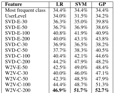
Table 3: 9-way classification accuracy on held-out data for our 3 methods. Textual features are ob-tained usingSVDor Word2Vec (W2V).E repre-sents embeddings, C clusters. The final number denotes the amount of clusters or the size of the embedding.

features at a time. Experiments combining features yielded only minor improvements. We apply com-mon linear and non-linear methods together with our proposedGPclassifier. The linear method is logistic regression (LR) with Elastic Net regulari-sation (Freedman, 2009) and the non-linear one is formulated by a Support Vector Machine (SVM) with an RBF kernel (Vapnik, 1998). The accuracy of our classifiers is measured on held-out data. Our data set is divided into stratified training (80%), validation (10%) and testing (10%) sets. The val-idation set was used to learn the LR and SVM hyperparameters, while the GP did not use this set at all. We report results using all three methods and all feature sets in Table 3.

We first observe that user level features (User-Level; see Section 4.1) are not useful for predicting the job class. This finding indicates that general so-cial behaviour or user impact are likely to be spread evenly across classes. It also highlights the diffi-culty of the task and motivates the use of deeper textual features.

ac-Rank Topic # Label Topic(most central words;most frequent words) MRRµ(l)

1 116 Arts lettering, steampunk;archival, stencil, canvas, minimalist, illustration, paintings, abstract, designs,art, design, print, collection, poster, painting, custom, logo,

printing, drawing .43 1.35

2 105 Health chemotherapy, diagnosis, disease, inflammation, diseases, arthritis, symptoms,patients, mrsa, colitis;risk, cancer, mental, stress, patients, treatment, surgery,

disease, drugs, doctor .20 2.76

3 153 Beauty Care exfoliating, cleanser, hydrating, moisturizer, moisturiser, shampoo, lotions,serum, moisture, clarins;beauty, natural, dry, skin, massage, plastic, spray,

facial, treatments, soap .19 3.69

4 21 _EducationHigher undergraduate, doctoral, academic, students, curriculum, postgraduate, enrolled,master’s, admissions, literacy;students, research, board, student, college,

education, library, schools, teaching, teachers .18 3.21 5 158 _EngineeringSoftware open-source, cisco, proprietary, avaya;integrated, data, implementation, integration, enterprise, configuration,service, data, system, services, access,

security, development, software, testing, standard .17 3.10 7 186 Football bardsley, etherington, gallas, heitinga, assou-ekotto, lescott, pienaar, warnock,ridgewell, jenas;van, foster, cole, winger, terry, reckons, youngster, rooney,

fielding, kenny .16 3.11

8 124 Corporate telecommunications, infrastructure, partnership;consortium, institutional, firm’s, acquisition, enterprises, subsidiary, corp,patent, industry, reports, global,

survey, leading, firm, 2015, innovation, financial .15 2.44 9 96 Cooking parmesan, curried, marinated, zucchini, roasted, coleslaw, salad, tomato, spinach,_{lentils;recipe, meat, salad, egg, soup, sauce, beef, served, pork, rice} .15 3.00 12 164 Elongated_{Words wooohooo, yaayyy;}yaaayy, wooooo, woooo, yayyyyy, yaaaaay, yayayaya, yayy, yaaaaaaay,_{wait, till, til, yay, ahhh, hoo, woo, woot, whoop, woohoo} .11 3.47 16 176 Politics nationalism, communism, apartheid;religious, colonialism, christianity, judaism, persecution, fascism, marxism,human, culture, justice, religion, democracy,

religious, humanity, tradition, ancient, racism .08 3.09 Table 4: Topics, represented by their most central and most frequent 10 words, sorted by their ARD lengthscale MRR across the nine GP-based occupation classifiers.µ(l)denotes the average lengthscale for a topic across these classifiers. Topic labels are manually created.

1 2 3 4 5 6 7 8 9

1

2

3

4

5

6

7

8

9

_0.0

0.2

0.4

0.6

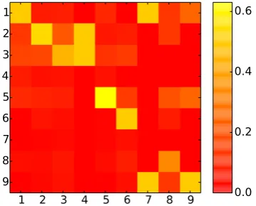
Figure 1: Confusion matrix of the prediction results. Rows represent the actual occupational class (C1– 9) and columns the predicted class.

curacy than the SVD on the NPMI matrix. This is consistent with previous work that showed the efficiency of word2vec and the ability of those em-beddings to capture non-linear relationships and syntactic features (Mikolov et al., 2013a; Mikolov et al., 2013b; Mikolov et al., 2013c).

LR has a lower performance than the non-linear

methods, especially when using clusters as features. GPs usually outperform SVMs by a small margin. However, these offer the advantages of not using the validation set and the interpretability properties we highlight in the next section. Although we only draw our focus on major occupational classes, the data set allows the study of finer granularities of oc-cupation classes in future work. For example, pre-diction performance for sub-major groups reaches 33.9% accuracy (15.6% majority class, 22 classes) and 29.2% accuracy for minor groups (3.4% major-ity class, 55 classes).

6.2 Error Analysis

that our model captures the general user skill level.

6.3 Qualitative Analysis

The word clusters that were built from a reference corpus and then used as features in the GP classi-fier, give us the opportunity to extract some qual-itative derivations from our predictive task. For the rest of the section we use the best performing model of this type (W2V-C-200) in order to anal-yse the results. Our main assumption is that there might be a divergence of language and topic us-age across occupational classes following previous studies in sociology (Bernstein, 1960; Bernstein, 2003). Knowing that the inferred GP lengthscale hyperparameters are inversely proportional to fea-ture (i.e. topic) relevance (see Section 5), we can use them to rank the topic importance and give answers to our hypothesis.

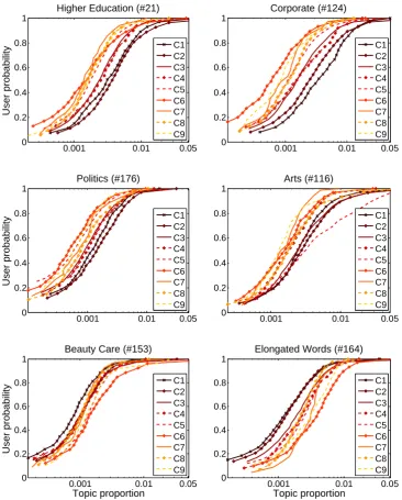
Table 4 shows 10 of the most informative top-ics (represented by the top 10 most central and frequent words) sorted by their ARD lengthscale Mean Reciprocal Rank (MRR) (Manning et al., 2008) across the nine classifiers. Evidently, they cover a broad range of thematic subjects, includ-ing potentially work specific topics in different do-mains such as ‘Corporate’ (Topic #124), ‘Software Engineering’ (#158), ‘Health’ (#105), ‘Higher Ed-ucation’ (#21) and ‘Arts’ (#116), as well as topics covering recreational interests such as ‘Football’ (#186), ‘Cooking’ (#96) and ‘Beauty Care’ (#153). The highest ranked MRR GP lengthscales only highlight the topics that are the most discrimina-tive of the particular learning task, i.e. which topic used alone would have had the best performance. To examine the difference in topic usage across occupations, we illustrate how six topics are cov-ered by the users of each class. Figure 2 shows the Cumulative Distribution Functions (CDFs) across the nine different occupational classes for these six topics. CDFs indicate the fraction of users having at least a certain topic proportion in their tweets. A topic is more prevalent in a class, if the CDF line leans towards the bottom-right corner of the plot.

‘Higher Education’ (#21) is more prevalent in classes 1 and 2, but is also discriminative for classes 3 and 4 compared to the rest. This is expected be-cause the vast majority of jobs in these classes require a university degree (holds for all of the jobs in classes 2 and 3) or are actually jobs in higher education. On the other hand, classes 5 to 9 have a similar behaviour, tweeting less on this topic. We

also observe that words in ‘Corporate’ (#124) are used more as the skill required for a job gets higher. This topic is mainly used by people in classes 1 and 2 and with less extent in classes 3 and 4, in-dicating that people in these occupational classes are more likely to use social media for discussions about corporate business.

There is a clear trend of people with more skilled jobs to talk about ‘Politics’ (#176). Indeed, highly ranked politicians and political philosophers are parts of classes 1 and 2 respectively. Neverthe-less, this pattern expands to the entire spectrum of the investigated occupational classes, providing further proof-of-concept for our methodology, un-der the assumption that the theme of politics is more attractive to the higher skilled classes rather than the lower skilled occupations. By examining ‘Arts’ (#116), we see that it clearly separates class 5, which includes artists, from all others. This topic appears to be relevant to most of the classifica-tion tasks and it is ranked first according to the MRR metric. Moreover, we observe that people with higher skilled jobs and education (classes 1–3) post more content about arts. Finally, we examine two topics containing words that can be used in more informal occasions, i.e. ‘Elongated Words’ (#164) and ‘Beauty Care’ (#153). We observe a similar pattern in both topics by which users with lower skilled jobs tweet more often.

1 2 3 4 5 6 7 8 9

1

2

3

4

5

6

7

8

9

_0.00

0.01

0.02

0.03

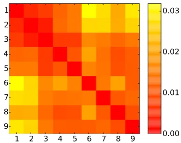
Figure 3: Jensen-Shannon divergence in the topic distributions between the different occupational classes (C1–9).

0.001 0.01 0.05 0

0.2 0.4 0.6 0.8 1

User probability

Higher Education (#21)

C1 C2 C3 C4 C5 C6 C7 C8 C9

0.001 0.01 0.05 0

0.2 0.4 0.6 0.8 1

Corporate (#124)

C1 C2 C3 C4 C5 C6 C7 C8 C9

0.001 0.01 0.05 0

0.2 0.4 0.6 0.8 1

User probability

Politics (#176)

C1 C2 C3 C4 C5 C6 C7 C8 C9

0.001 0.01 0.05 0

0.2 0.4 0.6 0.8 1

Arts (#116)

C1 C2 C3 C4 C5 C6 C7 C8 C9

0.001 0.01 0.05 0

0.2 0.4 0.6 0.8 1

Topic proportion

User probability

Beauty Care (#153)

C1 C2 C3 C4 C5 C6 C7 C8 C9

0.001 0.01 0.05 0

0.2 0.4 0.6 0.8 1

Topic proportion Elongated Words (#164)

C1 C2 C3 C4 C5 C6 C7 C8 C9

Figure 2: CDFs for six of the most important topics; the x-axis is on the log-scale for display purposes. A point on a CDF line indicates the fraction of users (y-axis point) with a topic proportion in their tweets lower or equal to the corresponding x-axis point. The topic is more prevalent in a class, if the CDF line leans closer to the bottom-right corner of the plot.

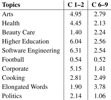
class pair. Figure 3 visualises these differences. There, we confirm that adjacent classes use simi-lar topics of discussion. We also notice that JSD increases as the classes are further apart. Two main groups of related classes, with a clear separation from the rest, are identified: classes 1–2 and 6–9. For the users belonging to these two groups, we compute their topic usage distribution (for the top topics listed in Table 4). Then, we assess whether the topic usage distributions of those super-classes of occupations have a statistically significant

Topics C 1–2 C 6–9

Arts 4.95 2.79

Health 4.45 2.13

Beauty Care 1.40 2.24 Higher Education 6.04 2.56 Software Engineering 6.31 2.54

Football 0.54 0.52

Corporate 5.15 1.41

Cooking 2.81 2.49

Elongated Words 1.90 3.78

Politics 2.14 1.06

Table 5: Comparison of mean topic usage for super-sets (classes 1–2 vs. 6–9) of the occupational classes; all values were multiplied by 103_{. The} dif-ference between the topic usage distributions was statistically significant (p <10−5_).

‘Corporate’ topic, whereas ‘Football’ registers the lowest distance.

7 Related Work

Occupational class prediction has been studied in the past in the areas of psychology and economics. French (1959) investigated the relation between var-ious measures on 232 undergraduate students and their future occupations. This study concluded that occupational membership can be predicted from variables such as the ability of subjects in using mathematical and verbal symbols, their family eco-nomic status, body-build and personality compo-nents. Schmidt and Strauss (1975) also studied the relationship between job types (five classes) and certain demographic attributes (gender, race, expe-rience, education, location). Their analysis identi-fied biases or discrimination which possibly exist in different types of jobs. Sociolinguistic and so-ciology studies deduct that social status is an im-portant factor in determining the use of language (Bernstein, 1960; Bernstein, 2003; Labov, 2006). Differences arise either due to language use or due to the topics people discuss as parts of various so-cial domains. However, a large scale investigation of this hypothesis has never been attempted.

Relevant to our task is a relation extraction ap-proach proposed by Li et al. (2014) aiming to ex-tract user profile information on Twitter. They used a weakly supervised approach to obtain informa-tion for job, educainforma-tion and spouse. Nonetheless, the information relevant to the job attribute

re-gards the employer of a user (i.e. the name of a company) rather than the type of occupation. In addition, Huang et al. (2014) proposed a method to classify Sina Weibo users to twelve predefined occupations using content based and network fea-tures. However, there exist significant differences from our task since this inference is based on a dis-tinct platform, with an ambiguous distribution over occupations (e.g. more than 25% related to me-dia), while the occupational classes are not generic (e.g. media, welfare and electronic are three of the twelve categories). Most importantly, the applied model did not allow for a qualitative interpreta-tion. Filho et al. (2014) inferred the social class of social media users by combining geolocation infor-mation derived from Foursquare and Twitter posts. Recently, Sloan et al. (2015) introduced tools for the automated extraction of demographic data (age, occupation and social class) from the profile de-scriptions of Twitter users using a similar method to our data set extraction approach. They showed that it is feasible to build a data set that matches the real-world UK occupation distribution as given by the SOC.

8 Conclusions

Acknowledgements

DP-P acknowledges the support from Templeton Religion Trust, grant TRT-0048. VL and NA ac-knowledge the support from EPSRC (UK) project EP/K031953/1. We thank Mark Stevenson for his critical comments on early drafts of this paper.

References

Faiyaz Al Zamal, Wendy Liu, and Derek Ruths. 2012. Homophily and Latent Attribute Inference: Inferring Latent Attributes of Twitter Users from Neighbors. InProc. of 6th International Conference on Weblogs and Social Media, pages 387–390.

Basil Bernstein. 1960. Language and social class.

British Journal of Sociology, pages 271–276. Basil Bernstein. 2003. Class, codes and control:

Ap-plied studies towards a sociology of language, vol-ume 2. Psychology Press.

Johan Bollen, Huina Mao, and Xiaojun Zeng. 2011. Twitter mood predicts the stock market. Journal of Computational Science, 2(1):1–8.

Gerlof Bouma. 2009. Normalized (pointwise) mutual information in collocation extraction. In Biennial GSCL Conference, pages 31–40.

D. John Burger, John Henderson, George Kim, and Guido Zarrella. 2011. Discriminating Gender on Twitter. InProceedings of the 2011 Conference on Empirical Methods in Natural Language Processing, EMNLP, pages 1301–1309.

Zhiyuan Cheng, James Caverlee, and Kyumin Lee. 2010. You are where you tweet: a content-based ap-proach to geo-locating twitter users. InProceedings of the 19th ACM Conference on Information and Knowledge Management, CIKM, pages 759–768. Trevor Cohn and Lucia Specia. 2013. Modelling

an-notator bias with multi-task gaussian processes: An application to machine translation quality estimation. In51st Annual Meeting of the Association for Com-putational Linguistics, ACL, pages 32–42.

Glen Coppersmith, Craig Harman, and Mark Dredze. 2014. Measuring post traumatic stress disorder in twitter. InInternational Conference on Weblogs and Social Media, ICWSM.

Renato Miranda Filho, Guilherme R. Borges, Jus-sara M. Almeida, and Gisele L. Pappa. 2014. Infer-ring user social class in online social networks. In

Proceedings of the 8th Workshop on Social Network Mining and Analysis, SNAKDD’14, pages 10:1– 10:5.

David Freedman. 2009.Statistical models: theory and practice. Cambridge University Press.

Wendell L French. 1959. Can a man’s occupation be predicted? Journal of Counseling Psychology, 6(2):95.

Mark Gibbs and David J. C. Mackay. 1997. Variational gaussian process classifiers. IEEE Transactions on Neural Networks, 11:1458–1464.

Brent Hecht, Lichan Hong, Bongwon Suh, and Ed H. Chi. 2011. Tweets from justin bieber’s heart: The dynamics of the location field in user profiles. In

Proceedings of the SIGCHI Conference on Human Factors in Computing Systems, CHI.

Yanxiang Huang, Lele Yu, Xiang Wang, and Bin Cui. 2014. A multi-source integration framework for user occupation inference in social media systems.

World Wide Web, pages 1–21.

William Labov. 2006. The Social Stratification of En-glish in New York City. Cambridge University Press, second edition.

Vasileios Lampos and Nello Cristianini. 2010. Track-ing the flu pandemic by monitorTrack-ing the Social Web. InProc. of the 2nd International Workshop on Cog-nitive Information Processing, pages 411–416. Vasileios Lampos and Nello Cristianini. 2012.

Now-casting Events from the Social Web with Statistical Learning. ACM Transactions on Intelligent Systems and Technology, 3(4):72:1–72:22.

Vasileios Lampos, Daniel Preot¸iuc-Pietro, and Trevor Cohn. 2013. A user-centric model of voting in-tention from Social Media. In Proceedings of the 51st Annual Meeting of the Association for Compu-tational Linguistics, ACL, pages 993–1003.

Vasileios Lampos, Nikolaos Aletras, Daniel Preot¸iuc-Pietro, and Trevor Cohn. 2014. Predicting and char-acterising user impact on Twitter. InProceedings of the 14th Conference of the European Chapter of the Association for Computational Linguistics, EACL, pages 405–413.

Omer Levy and Yoav Goldberg. 2014. Neural word embeddings as implicit matrix factorization. In Ad-vances in Neural Information Processing Systems, NIPS, pages 2177–2185.

Jiwei Li, Alan Ritter, and Eduard H. Hovy. 2014. Weakly supervised user profile extraction from twit-ter. InProceedings of the 52nd Annual Meeting of the Association for Computational Linguistics, ACL, pages 165–174.

Christopher D. Manning, Prabhakar Raghavan, and Hinrich Sch¨utze. 2008. Introduction to Information Retrieval. Cambridge University Press.

Tomas Mikolov, Ilya Sutskever, Kai Chen, Greg Cor-rado, and Jeffrey Dean. 2013b. Distributed represen-tations of words and phrases and their composition-ality. InAdvances in Neural Information Processing Systems, NIPS, pages 3111–3119.

Tomas Mikolov, Wen tau Yih, and Geoffrey Zweig. 2013c. Linguistic regularities in continuous space word representations. InProceedings of the 2010 annual Conference of the North American Chap-ter of the Association for Computational Linguistics, NAACL, pages 746–751.

Thomas P. Minka. 2001. Expectation propagation for approximate bayesian inference. InProceedings of the 17th Conference in Uncertainty in Artificial In-telligence, UAI ’01.

Radford M. Neal. 1996.Bayesian Learning for Neural Networks. Springer-Verlag New York, Inc.

Radford M. Neal. 1999. Regression and classification using gaussian process priors. Bayesian Statistics 6, pages 475–501.

Andrew Y. Ng, Michael I. Jordan, and Yair Weiss. 2002. On spectral clustering: Analysis and an algo-rithm. InAdvances in Neural Information Process-ing Systems, NIPS, pages 849–856.

Marco Pennacchiotti and Ana-Maria Popescu. 2011. A machine learning approach to twitter user classifi-cation. ICWSM, pages 281–288.

Tamara Polajnar, Simon Rogers, and Mark Girolami. 2011. Protein interaction detection in sentences via gaussian processes; a preliminary evaluation. Inter-national Journal of Data Mining and Bioinformatics, 5(1):52–72.

Daniel Preot¸iuc-Pietro and Trevor Cohn. 2013. A tem-poral model of text periodicities using Gaussian Pro-cesses. EMNLP.

Daniel Preot¸iuc-Pietro, Sina Samangooei, Trevor Cohn, Nicholas Gibbins, and Mahesan Niranjan. 2012. Trendminer: An architecture for real time analysis of social media text. In Workshop on Real-Time Analysis and Mining of Social Streams (RAMSS), ICWSM.

Delip Rao, David Yarowsky, Abhishek Shreevats, and Manaswi Gupta. 2010. Classifying Latent User At-tributes in Twitter. In Proceedings of the 2nd In-ternational Workshop on Search and Mining User-generated Contents, SMUC, pages 37–44.

Carl Edward Rasmussen and Christopher K. I. Williams. 2006. Gaussian Processes for Machine Learning. The MIT Press.

Adam Sadilek, Henry Kautz, and Vincent Silenzio. 2012. Modeling Spread of Disease from Social In-teractions. InProc. of 6th International Conference on Weblogs and Social Media, pages 322–329.

Peter Schmidt and Robert P Strauss. 1975. The predic-tion of occupapredic-tion using multiple logit models. In-ternational Economic Review, 16(2):471–86. Jianbo Shi and Jitendra Malik. 2000. Normalized cuts

and image segmentation. Transactions on Pattern Analysis and Machine Intelligence, 22(8):888–905. Luke Sloan, Jeffrey Morgan, Pete Burnap, and Matthew

Williams. 2015. Who tweets? Deriving the demo-graphic characteristics of age, occupation and so-cial class from twitter user meta-data. PloS one, 10(3):e0115545.

Edward Snelson and Zoubin Ghahramani. 2006. Sparse gaussian processes using pseudo-inputs. In

Advances in Neural Information Processing Systems, NIPS, pages 1257–1264.

Andranik Tumasjan, Timm Oliver Sprenger, Philipp G Sandner, and Isabell M Welpe. 2010. Predicting Elections with Twitter: What 140 Characters Reveal about Political Sentiment. In Proc. of 4th Inter-national Conference on Weblogs and Social Media, pages 178–185.

Vladimir N Vapnik. 1998. Statistical learning theory. Wiley, New York.

Ulrike von Luxburg. 2007. A tutorial on spectral clus-tering.Statistics and computing, 17(4):395–416. Christopher K.I Williams and David Barber. 1998.

Bayesian classification with gaussian processes.