Munich Personal RePEc Archive
Energy Conservation, Fossil Fuel
Consumption, CO2 Emission and
Economic Growth in Indonesia
Erdyas Bimanatya, Traheka and Widodo, Tri
Economics Department, Faculty of Economics, Gadjah Mada
University
28 June 2017
Energy Conservation, Fossil Fuel Consumption, CO2 Emission and Economic Growth in Indonesia
by:
Traheka Erdyas Bimanatya
and
Tri Widodo
Economics Department, Faculty of Economics and Business, Gadjah Mada University
Coresponding author. Current Mailing Address: Faculty of Economics and Business, Gadjah Mada
Energy Conservation, Fossil Fuel Consumption, CO2 Emission and Economic Growth in Indonesia
Abstract
This paper discusses the relationship between fossil fuel consumption, carbon dioxide emissions and economic growth for the period of 1965-2012 in Indonesia by applying Vector Error Correction Model (VECM) Granger causality. This paper also estimate the effect of energy conservation policy that has already adopted the National Energy Conservation Master Plan (RIKEN 2005) by Indonesian Government to the pattern of energy consumption in Indonesia from 2014 until 2030. Empirical results show that in the short-run there are unidirectional Granger causalities running from coal consumption to economic growth (growth hypothesis) and from economic growth to oil consumption (conservation hypothesis). However, in the long run the results suggest unidirectional Granger causality only running from oil consumption to economic growth and CO2 emissions. Thus, Indonesia should adopts different policies for
each type of energies in order to maintain the economic growth while the effort of reducing fossil fuel consumption is in progress. The projection results imply that Indonesia government should revise the energy efficiency targets in RIKEN 2005 since the result of LEAP Projection based on RIKEN target shows a lower energy saving rate (17.32 percent) compared to the target (18 percent).
Keywords:Fossil Fuel Consumption; CO2 Emission; Economic Growth.
JEL classification: Q43; Q53; O44
1. Introduction
Entering the 21st century, fossil fuels are still the dominant source of
energy in the world energy demand. Compared with the energy demand
conditions a few decades ago, the relative consumption patterns do not change
much. In 1973, three-quarters (75.8 percent) source of energy consumed by the
world comes from fossil fuels. Consumption of petroleum that time nearly half the
world's energy consumption is 48.1 percent. Natural gas and coal accounted for
Petroleum is still a fossil fuel that is the most widely consumed is equal to 40.8
percent of total world energy consumption, and then followed in succession by
15.5 percent natural gas, and coal at 10.1 percent. (IEA, 2013a).
In an effort to maintain economic growth, energy consumption is needed
to change the basic ingredient materials into goods and services that benefit
society (Budiarto, 2013). By sector, the use of fossil fuel users are divided into
several sectors, such as transport, industry, agriculture, commercial and public
services, households and other sectors. In 2011, the transport sector absorbed 62.3
percent of petroleum consumption while the industrial sector absorbed 36.7
percent of natural gas consumption and 80.7 percent of world coal consumption
(IEA, 2013a).
World's dependence on fossil fuels have serious implications for the
environment. Emissions of carbon dioxide (CO2) that is released by fossil fuels is
a major cause of global warming (Ozturk and Acaravci, 2010; Zhang and Cheng,
2009). In 2011, as many as 83 percent of greenhouse gases 93 percent in the form
of CO2 emissions come from the energy sector. In the energy sector alone most of
the CO2 emissions produced by the process of carbon oxidation (combustion) of
the fuel (IEA, 2013b).
Until now, a wide variety of empirical studies have been conducted by
academics and practitioners to explain the relationship between energy
consumption, environmental pollution and economic growth in the domestic and
regional levels. Various empirical studies have shown mixed results because of
analysis used by the researchers (Hwang and Yoo, 2012). Therefore, further
studies with the object of study, the period of the study, and different methods of
analysis needs to be done to prove the relationship of the above three.
In this study, Indonesia was chosen as a case study object. This selection
was based on three things. First, the primary energy consumption patterns in
Indonesia from 1965 until 2012, still dominated by fossil fuels as seen in Figure 3.
The share of fossil fuel consumption to primary energy in Indonesia as an annual
average (1965-2012) is 96.5 percent, never even reached 98.98 percent in 1981.
Second, the level of CO2 emissions in Indonesia continued to show a rising trend.
In 1965, Indonesia has a CO2 emission level of only 20.35 million metric tons but
by 2012 had reached 495.21 million metric tons, an increase of 2,333 percent.
United States Energy Information Administration (EIA) puts Indonesia as the
seventeenth ranked emitters of CO2 in the year 2011. Third, Indonesia is one of
the developing countries which are members of the G20 forum and has the fourth
largest population in the world after China, India, and the United States. This
Figure 1 Fossil Fuel Consumption share of Indonesia to the Primary Energy, 1965-2012
Source: BP Statistical Review of World Energy, 2014
By paying attention to three things above, research on the inter-relationship
between the consumption of fossil fuels, the level of CO2 emissions, and
economic growth in Indonesia to be relevant to be done. In addition to the
upcoming projected levels of energy consumption, especially when the
government implemented a policy of energy conservation, it is necessary to know
the change in consumption levels that may occur. This paper is addressed to
answer critical questions as follow: Based on the background and formulation of
the problem described by the researchers, the research question is formulated as
follows: First, how causal relationship between the level of consumption of fossil
fuels (petroleum, coal, and natural gas), the rate of economic growth and the level
of CO2 emissions in Indonesia? How does the impact of the implementation of
energy conservation policy in Indonesia against the energy consumption levels of
2. Literature Study
Tiwari (2011 and 2010) states that there are four kinds of hypotheses that
explain the relationship between energy consumption and economic growth. The
first hypothesis, Growth Hypothesis, expressed energy consumption directly
influence the rate of economic growth. The more energy that is consumed as
inputs in the production process, the more the output produced so that the
economic growth rate is also higher. The second hypothesis, Conservation
Hypothesis, otherwise stated rate of economic growth determine the extent of the
energy consumed by the public. Thus, a country's policy to limit its energy
consumption levels will not reduce economic growth.
The third hypothesis, Feedback Hypothesis, stating the level of energy
consumption and economic growth are interdependent. That means between the
two influence each other or with other words having a two-way causality. Latter
hypothesis, Neutrality Hypothesis, states that there is a relationship of mutual
influence between the levels of energy consumption with economic growth so that
it can be interpreted both variables are independent of each other.
The fourth hypothesis above is empirical proof of the theory of economic
growth that became mainstream in the study of energy economics, namely the
Augmented Solow Growth Model. The model is the development of a model of
economic growth created by Robert Solow (1956).
Various empirical studies have been conducted to determine the
relationship between economic activity and environmental quality of life. Most of
theoretical basis as in Choi et al. (2010), Granados and Carpintero (2009), and
Azomahou et al. (2005). Based on the concept of EKC, the relationship of
economic activity, represented by per capita income, and environmental
conditions, represented the level of pollutant emissions, can be illustrated by the
graph in the form of "U" upside down (inverted-U). EKC concept itself comes
from an article written by Gene M. Grossman and Alan B. Krueger in 1991 and
then popularized by the World Bank in its World Development Report 1992
[image:8.595.169.505.326.568.2](Stern, 2003).
Figure 2. Environmental Kuznets Curve Source: Stern (2004)
The relationship between environmental degradation with the economic
activity later clarified by the model developed by several researchers. One is the
model proposed by Brock and Taylor (2004). According to them, the amount of
there are efforts to control (abatement) of the manufacturer. Mathematical
notation of the model is as follows:
Error! Reference source not found. (1)
The second line of equation (1) shows that the level of aggregate
emissions (E) is the reduction of the level of emissions generated by economic
activity (ΩF) with emission levels that were reduced by the manufacturer through
control efforts (ΩA). The level of control efforts (A) itself is a function of
aggregate economic activity scale (F) and the economic activity that is used for
emission control measures (FA). In addition, the last line can be seen that the level
of aggregate emissions are generally influenced by two things: the scale of
aggregate economic activity (F) and the production technology is denoted by e
(θ).
3. Methodology 3.1. Model
By combining the two models above study, researchers formulate a mathematical
model to explain the relationship between economic growth, fossil energy
(2)
Real GDP is used in the model to explain the economic growth variable (Y).
While variable consumption of fossil energy (FE) is divided into three types,
namely energy consumption of petroleum, coal, and natural gas. The division is
intended to determine the relationship of each individual type of fossil energy to
other variables. Value of all the variables are expressed in natural logarithm form
large elasticity between variables that can be known. In addition, a dummy
variable was also added in 1998 to capture changes in the trend of the data before
and after the economic crisis of 1997-1998.
Researchers using the Vector Error Correction Model (VECM) to examine
the relationship above five variables. Model specification testing in this study are
as follows:
(2)
(3)
(4)
(5)
The notation C represents the level of CO2 emissions, the notation G is the
number of real GDP, E1 is the amount of petroleum consumption, E2 is the
amount of natural gas consumption, and E3 is the amount of coal consumption.
Dummy variable is explained by the 1997-1998 economic crisis notation D1998.
As for seeing the changes in the pattern of consumption of fossil fuels in
society when the government implemented a policy of energy conservation,
researchers using LEAP projection model with a focus on demand modules. The
time span chosen for the projection of energy demand is ranging from 2012 to
2025 according to the Energy Vision 25/25, announced by the government.
Graphically the model projections for the final energy demand module Indonesia
[image:11.595.160.499.424.678.2]is structured as follows:
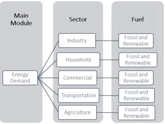
Figure 3. LEAP Projection Model of Indonesia Energy Final Demand, 2012 – 2025
Request module is divided into five sectors namely industrial sector
energy users, household, commercial, transportation and others. The agricultural
sector also includes forestry and fisheries. Total energy demand in each sector is
further divided into four types of energy, namely oil, coal, natural gas, and
energy-energy from renewable sources. Types of renewable energy in this study
follows the classification of the IEA, namely nuclear power, geothermal, hydro,
biofuels, and others. In addition, historical data from 2005 to 2011 was also added
in the model to see the trend of the development of sectoral energy demand in
Indonesia. As a proxy for energy demand, the researchers used data types and
energy consumption per user per sector published by the IEA.
3.2. Limitations of Study
This study is limited in several respects. First, the time period of data used
in this study are in the period 1965 through 2012 Secondly, the type of energy that
covers the entire studied the fossil fuels oil, coal, and natural gas. Third, this study
only looked at the relationship between the level of consumption of fossil fuels
with CO2 emission levels and economic growth in Indonesia. Fourth, the
projected level of energy consumption is only done in the public sector, industry,
households, transport, commercial, and agriculture (including forestry and
fisheries).
3.3. Hypothesis
In this study, the hypotheses used are as follows: Firstly, the rate of
consumption of fossil energy (oil, coal, and natural gas) has a causal relationship
(oil, coal, and natural gas) has a causal relationship to the level of CO2 emissions
in Indonesia. Economic growth has a causal relationship to the level of CO2
emissions in Indonesia. Energy conservation policies influence the change in the
pattern of consumption of fossil fuels Indonesian society
3.4. VECM Granger Causality
VECM first introduced by Sargan (1964) and later developed by
Engle and Granger (1987) and Johansen (1988). Also known as the VECM
Cointegrating Vector Autoregression models (CIVAR) or VAR which is restricted
(restricted VAR) because VECM using variables and apply the concept of
cointegrating error correction (Error Correction) in the estimation process.
Widarjono (2009) states that the application of the concept of error correction
aims to restrict the behavior of a long-term relationship between variables in order
to converge to the cointegration relationship while still allowing dynamic changes
in the short term. Both the concept of co-integration and error correction is used to
prevent the occurrence of spurious regression (Lauridsen, 1998).
Procedurally, VECM chosen as the model estimation when the unit root
test indicates the variables that exist largely stationary at level but cointegration
test results indicate the presence of co-integration or in other words there is a
theoretical relationship between variables. According Obayelu and Salau (2010),
VECM assumes these variables are linearly adjusted to balance the long-term.
While Engle and Granger (1987) concluded that the change in the dependent
well as great value for Error Correction Term (ECT). The ECT itself shows the
long-term coefficients of the model.
Based on the above explanation, VECM can be formulated as follows
(Suryaningsih et al., 2012):
Error! Reference source not found. (7)
with the notation Yt show (k x 1) vector of endogenous variables, α is the
adjustment coefficient that measures the level of the endogenous variable speed
adjustment in the long run i, β is the cointegration vector, Dt is a vector of
deterministic terms, Γ1 ... p is (k x k) matrix of coefficients, C* is the matrix
associated with deterministic terms are used in the model as a constant, with a
trend or seasonal dummy; and Ut is the reduced form disturbance. As indicated by
the combined ECT variable notation β and Yt-1. Harris (1995) in Ajija et al. (2011)
also formulate VECM number 20 in the form of the following equation:
(8)
In the analysis, VECM models often also used in conjunction with the Granger
Causality test so this approach is often referred to as the VECM Granger
Causality. This approach has the distinction of the causality test proposed by
Granger (1969). In addition to providing information towards the relationship
between variables, this approach also explains the relationship time horizon is
short term or long term. Tiwari (2011) revealed that the long-term relationship can
be explained by the significance of the lagged ECT while the short-term
relationship can be seen from the significance of the coefficient of the first
difference of the independent variables. Mathematical modelling VECM Granger
Causality as follows:
Error! Reference source not found. (9)
Error! Reference source not found. (10)
The above model is used to test the hypothesis that the variable X determines the
value of the variable Y. The null hypothesis of equation (9) is Error! Reference source not found.and equation (10) is Error! Reference source not found.. Thus, if the null hypothesis is rejected fails equation (9) it can be concluded that
the variable Y does not affect the variable X. Conversely, if the null hypothesis is
rejected, the equation (10) fails the conclusion is no effect of variable X on
variable Y. If the models using only a single lag, then hypothesis testing can be
done by t-test. However, if the variables in the model using more than one lag (lag
such as two, or three lag), the significance test used was the F-test. Similarly, the
same applies to the hypothesis test for the long-term variable in the second
equation ECT VECM Granger Causality.
4.4. Long-range Energy Alternatives Planning (LEAP)
LEAP The term actually refers to a software (software) computer
developed by the Stockholm Environment Institute first time in 1981 aims to
facilitate the development of LEAP experts in assessing the impact of energy and
environmental policy in a particular region over a range of periods. In addition,
production and mitigation of greenhouse gas emissions in an economy. Since
1981, LEAP has been improved several times including in 2000, 2006, 2008 and
2014 in the last year doing modeling, LEAP uses accounting approach. Total
demand and total energy supply is calculated by summing the usage and supply of
each type of energy in each sector or activity (Wintarro, 2008).
There are four main modules in the LEAP module Assumptions Key (Key
Assumptions), Demand (Demand), Transformation (Transformation), and
Resources (Resources). Module generally contains key assumptions of
macroeconomic variables that affect the value of the variables in other modules
such as population and GDP. The module is used to accommodate the demand
variables disaggregate energy consumption. Mathematically, the energy demand
is defined as follows (Help for LEAP, 2014):
Energy consumption = activity level x energy intensity (11)
Transformation module is useful to calculate the amount of energy supply, both
primary and secondary, through energy input-output tables. The resource module
summarizes the results of a calculation module based on the type of energy
transformation separately.
In addition to the main module, LEAP also has three additional modules
that are complementary to the main module Difference Statistics (Statically
Differences), Changes in Stock (Stock Changes), and the impact of non-energy
sector (Non-Energy Sector Effects). Module contains statistical difference
assumptions statistical difference between the demand and supply of energy due
accommodate the assumptions change in energy reserves between periods.
Modules incorporate the impact of non-energy sectors of the variables that capture
the energy production and consumption externalities such as air pollution level
and the number of patients with respiratory tract infections.
4. Results and Analysis
As shown in Figure 1, in term of primary energy, Indonesia still heavily
relies on fossil fuel. This paper evaluates the relation between the fossil fuel
consumption, economic growth, and pollution rate based on the annual data from
World Bank and British Petroleum. The variable of fossil fuel consumption are
divided into three energy type from BP s (Oil, Natural Gas, and Coal). Those data,
together with CO2 emissions, are taken Statistical Review of World Energy 2013
and measured in million tons oil equivalent (Mtoe) for energy consumption and
million tons carbon dioxide for other. To make a proxy for real economic growth,
this paper uses Constant Price 2005 GDP measured in US dollars obtained from
the World Bank.
Table 1 illustrates the descriptive statistical analysis of the data. All
variables are expressed in logarithmic form to standardize the unit of
measurement. The econometric model also added dummy variable for 1998 crisis
(0 for period before 1998, 1 for otherwise) to solve normality problem in data
analysis.
Variable LCO2 LGDPR LOIL LGAS LCOAL
Mean 4.729735 25.52754 3.209114 2.130647 0.521503
Median 4.842086 25.60484 3.289876 2.637422 1.078201
Maximum 6.204962 26.78115 4.271095 3.591818 3.919991
Minimum 2.954910 24.05553 1.740466 -0.693147 -2.302585
Std. Dev. 1.045926 0.819352 0.821498 1.419775 2.309221
Skewness -0.334727 -0.292666 -0.476576 -0.804840 -0.011349
Kurtosis 1.805448 1.845921 1.895687 2.184273 1.421944
Jarque-Bera 3.750251 3.349024 4.256011 6.512963 4.981553
Probability 0.153336 0.187400 0.119075 0.038524 0.082846
Source: calculated from WB database and BP Statistical Review of World Energy, 2014
4.1. Unit Roots
This paper applies Augmented Dicky-Fuller (ADF) and Phillips-Perron
(PP) test to investigate the existence of unit roots. By assuming that the test model
has a trend and intercept, both the ADF and PP tests show that all variables are
not stationary in levels. In contrast, all variables are one percent significant in first
difference or in other words, the null hypothesis that the data contains time series
unit root can be rejected. Therefore it can be concluded that the variables in this
[image:18.595.114.519.113.308.2]paper are integrated in the I(1).
Variable
Level First Difference
t-stat Adj. t-stat t-stat Adj. t-stat
LCO2 -0.55633 (0.9770) -0.849924 (0.9531) -6.374173* (0.0000) -6.380551* (0.0000)
LGDPR -1.65625 (0.7544) -1.249867 (0.8879) -5.221177* (0.0005) -5.207384* (0.0005)
LOIL -0.32116 (0.9877) -0.635945 (0.9719) -6.151965* (0.0000) -6.146971* (0.0000)
LGAS -0.72075 (0.9645) -0.904911 (0.9468) -4.60061* (0.0034) -7.337728* (0.0000)
LCOAL -2.1657 (0.4969) -2.165703 (0.4969) -6.891926* (0.0000) -6.872561* (0.0000)
rce: calculated from WB database dan BP Statistical Review of World Energy, 2014
Note: * significant at 1 per cent
4.2. Determining the Optimal Lag
Determination of the optimal lag VAR models using a variety of
criteria summarized in table 3. Final Prediction Error (FPE) criteria, Schwarz
Information Criterion (SIC), Hannan-Quinn Information Criterion (HQ)
recommend one lag. While the criteria of sequential modified LR test statistic
(LR) and the Akaike Information Criterion (AIC) shows the optimal lag VAR
[image:19.595.164.517.115.347.2]located on the lag of four.
by Using Various Criterion
Source: calculated from WB database dan BP Statistical Review of World Energy, 2014
Note: * recommended lag by criterion
4.3. Co-integration test and Vector error correction model
Table 4 presents the result of the Johansen co-integration test as
determined by the Max-Eigenvalue and trace methods. This cointegration test
uses optimal VAR lag-1 as an interval limit of test lag. Both the maximum
eigenvalue and trace statistics show significant value at five per cent, so the null
hypothesis that there are only at most two cointegrating equations can be rejected.
Thus the five variables have three cointegrating equation at a maximum lag of
[image:20.595.135.549.134.266.2]three periods.
Table 4 Results of the Johansen co-integration test by the max-eigenvalue and trace methods
Lag LogL LR FPE AIC SC HQ
0 83.21482 NA 2.47E-08 -3.32795 -2.92245 -3.17757
1 330.506 415.8987 1.02e-12* -13.4321 -12.01285* -12.90577*
2 345.4332 21.71241 1.71E-12 -12.9742 -10.5413 -12.072
3 369.9727 30.11658 2.01E-12 -12.9533 -9.50657 -11.6751
4 414.0967 44.12400* 1.12E-12 -13.82258* -9.3621 -12.1684
Rank Eigenvalue Max-Eigen Statistics
Trace Statistics
r = 0 * 0.936920 121.5874 (0.0000)
217.4141 (0.0000)
r ≤ 1 * 0.663914 47.97707
(0.0003)
95.82674 (0.0000)
r ≤ 2 * 0.465032 27.52415
(0.0296)
47.84968 (0.0149)
r ≤ 3 0.258682 13.17032
(0.3145)
20.32553 (0.2099)
r ≤ 4 0.150084 7.155202
(0.3286)
[image:20.595.123.523.575.741.2]Source: calculated from WB database dan BP Statistical Review of World Energy, 2014
Note: * significant at 5 per cent; number in parentheses ( ) indicates the magnitude of P-Value for each statistics.
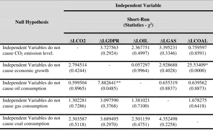
Table 5 and table 6 illustrate the result of short-run and long-run
multivariate causality tests based on the vector error correction model (VECM).
This paper uses a significance of 10 percent as a limitation for the causality test in
both tables. In the short run there are two significant unidirectional granger
causalities from coal consumption to economic growth (growth hypothesis) and
[image:21.595.108.544.357.622.2]also from economic growth to oil consumption (conservation hypothesis).
Table 5. Short-Run Multivariate Causality based on VECM
Source: calculated from WB database dan BP Statistical Review of World Energy, 2014
Note: *,**,*** significant at 1, 5, 10 per cent respectively; number in parentheses ( ) indicates the magnitude of P-Value for each statist
While for the long run, there are several significant variables and have a
strong causality. First, unidirectional granger causalities of petroleum
Null Hypothesis
Independent Variable
Short-Run (Statistics - χ2)
∆LCO2 ∆LGDPR ∆LOIL ∆LGAS ∆LCOAL
Independent Variables do not cause CO2 emission level.
- 3.727563
(0.2924) 2.367751 (0.4997) 3.395231 (0.3346) 0.759597 (0.8591)
Independent Variables do not cause economic growth
2.794514 (0.4244)
- 0.057297
(0.9964)
2.928688 (0.4028)
25.53409* (0.0000)
Independent Variables do not cause oil consumption
0.599504 (0.8965)
7.882641** (0.0485)
- 0.655319 (0.8837)
0.639562 (0.8873)
Independent Variables do not cause gas consumption
1.302281 (0.7286) 3.097590 (0.3768) 1.381021 (0.7100)
- 1.678275 (0.6418)
Independent Variables do not cause coal consumption
2.303587 (0.5118) 3.689495 (0.2970) 2.501159 (0.4751) 4.352498
consumption to economic growth and CO2 level. Second, bidirectional granger
causalities of coal consumption to economic growth and CO2 level. Third,
bidirectional granger causalities of gas consumption to economic growth and CO2
level. Fourth, bidirectional granger causality of economic growth to the level of
[image:22.595.66.570.283.555.2]CO2.
Table 6. Long-Run Multivariate Causality based on VECM
Source: calculated from WB database dan BP Statistical Review of World Energy, 2014
Note: *,**,*** significant at 1, 5, 10 per cent respectively; number in parentheses ( ) indicates the magnitude of P-Value for each statistics.
4.4. Energy Consumption Projection Using LEAP
This paper uses two kinds of projection scenarios. The first scenario is Business as
Usual (BAU) scenario. This scenario assumes no change in energy policy in the
future. The second scenario is the implementation of the National Energy
Conservation Master Plan (RIKEN) 2005 by the government scenario. RIKEN
Null Hypothesis
Joint Statistic - χ2 Statistic - χ2
∆LCO2 ∆LGDPR ∆LOIL ∆LGAS ∆LCOAL
Independent Variables do not cause CO2
emission level
- 13.62879** (0.0341) 11.99765*** (0.0620) 12.12108*** (0.0593) 8.811611 (0.1845) 8.654258** (0.0343) Independent Variables do not cause economic growth
176.3363*
(0.0000) -
183.9862* (0.0000) 172.9715* (0.0000) 184.8821* (0.0000) 163.0336* (0.0000) Independent Variables do not cause oil consumption
1.625955 (0.9507)
9.367858
(0.1539) -
2.068045 (0.9133) 2.027601 (0.9171) 1.465999 (0.6901) Independent Variables do not cause gas consumption 20.75767* (0.0020) 20.45929* (0.0023) 18.82662*
(0.0045) -
24.70850* (0.0004)
18.44682* (0.0004)
Independent Variables do not cause coal consumption 7.913258 (0.2445) 12.97702** (0.0434) 9.749208 (0.1356) 8.505578
(0.2034) -
scenario assumes in 2025 each sector can do a certain level of energy efficiency.
In detail, the potential assumption of energy efficiency in each sector are
[image:23.595.133.493.195.326.2]presented in the following table:
Table 7. Potential and Energy Efficiency Target in 2025 Sector Energy Efficiency
Potential (%)
Energy Efficiency Target in 2025(%)
Industry 10-30 17
Commercial 10-30 15
Transportation 15-35 20
Household 15-30 15
Agriculture 15-30 0
Source: Draft of RIKEN 2005-Energy Conservation Directorate, ESDM Ministry
RIKEN scenario refers to the Vision 25/25 whose goal is achieving a
reduction in energy consumption by 18 percent from the BAU scenario by 2025
through energy conservation activities. Determination of the energy efficiency
target figure itself is one of the programs to achieve the realization of the Vision
25/25. The projection of energy consumption level in 2025 with the BAU scenario
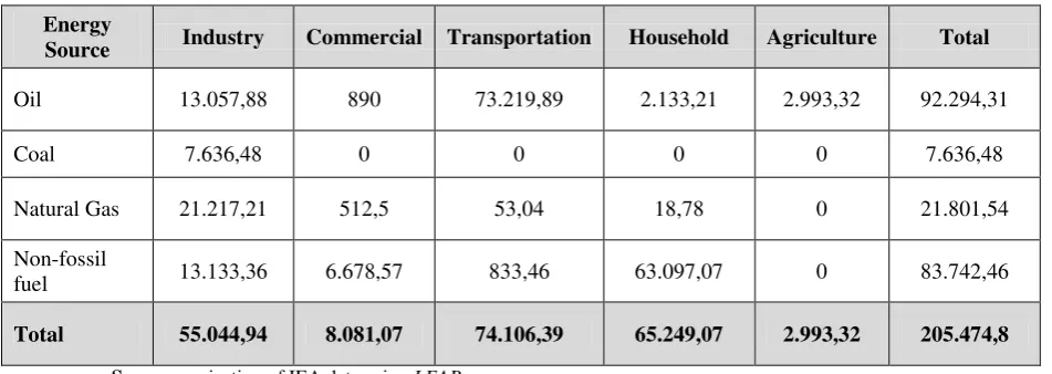
is shown in the table 8 below:
Table 8. Projection of Indonesia Energy Consumption Level in 2025 (Ktoe)
Source: projection of IEA data using LEAP
Energy
Source Industry Commercial Transportation Household Agriculture Total
Oil 13.057,88 890 73.219,89 2.133,21 2.993,32 92.294,31
Coal 7.636,48 0 0 0 0 7.636,48
Natural Gas 21.217,21 512,5 53,04 18,78 0 21.801,54
Non-fossil
fuel 13.133,36 6.678,57 833,46 63.097,07 0 83.742,46
[image:23.595.63.539.565.734.2]Based on the projection results, if government implements RIKEN
2005 scenario in 2025, there will be a 35.58 Mtoe energy saving with potential
energy efficiency interval of 27.66 to 65.35 Mtoe. That figures by percentage are
equal with 17.32 per cent and 13.46 - 31.80 per cent of BAU scenario energy
consumption level respectively. As shown in the table above, the largest energy
saving belongs to transportation sector (14.82 Mtoe), then followed by household
sector (9.79 Mtoe), industry (9.36 Mtoe), and commercial (1.62 Mtoe). In the
agricultural sector, the Government does not establish special targets so that the
amount of energy consumption in the agricultural sector in RIKEN scenario same
with BAU scenario.
6. Conclusions
This paper evaluates the long run and short run causality issues between fossil
fuel consumption (oil, natural gas, and coal), CO2 emissions, and economic
growth in Indonesia by using Vector Error Correction Model (VECM) Granger
Causality for the period of 1965-2012. Empirical results suggest each types of
fossil fuel has different causality direction both in the long run and short run. The
main results for the existence and direction of VECM granger causality are as
follows: First, in the short-run there are unidirectional Granger causalities running
from coal consumption to economic growth (growth hypothesis) and from
economic growth to oil consumption (conservation hypothesis). Second, in the
long run the results suggest unidirectional Granger causality (growth hypothesis)
emissions while other variables have bidirectional Granger causality (feedback
hypothesis).
This paper also projects the effect of energy conservation policy that has
already adopted (RIKEN 2005) by Indonesian Government to the pattern of
energy consumption in Indonesia from 2014 until 2030. The projection results
imply that Indonesia government should revise the energy efficiency targets at
RIKEN (National Energy Conservation Master Plan) 2005 since the result of
LEAP Projection based on RIKEN target shows a lower energy saving rate (17.32
percent) compared to the Vision 25/25 target (18 percent).
References
Ahmad, S., Muhammad, S., Shabbir, R. and Wahid, A. (2010). “Predicting Future Energy Requirements of Punjab (Pakistan) Agriculture Sector Using LEAP Model.”World Applied Sciences Journal, 8(7), pp.833-838.
Ajija, S.R., Sari, D.W., Setianto, R.H., and Primanti, M.R. 2011. Cara Cerdas Menguasai EViews. 1st ed. Jakarta: Salemba Empat, pp.191-192.
Alkhathlan, K., Alam, M. Q.and Javid, M. (2012).“Carbon Dioxide Emissions, Energy Consumption and Economic Growth in Saudi Arabia: AMultivariate Cointegration Analysis.”British Journal Of Management dan Economics, 2 (4).
Arrow, K., Bolin, B., Costanza, R., Dasgupta, P., Folke, C., Holling, C. S., Jansson, B., Levin, S., M"Aler, K., Perrings, C. and Others (1995). “Economic Growth, Carrying Capacity, and The Environment.” Ecological Economics, 15 (2), pp. 91-95.
Asia-Pacific Economic Cooperation.(2012). Peer Review on Energy Efficiency in Indonesia: Final Draft Report.
Ayres, R. U. and Warr, B. (2005).“Accounting for Growth: The Role of Physical Work.”Structural Change And Economic Dynamics, 16 (2), pp. 181--209.
Azomahou, T., Laisney, F. and Van, P. N. (2005).“Economic Development and CO2 Emissions: A Nonparametric Panel Approach.”ZEW Discussion Paper,
Berndt, E. R. and Wood, D. O. (1975).”Technology, Prices, and The Derived Demand for Energy.”The Review Of Economics And Statistics, pp. 259-268.
British Petroleum. (2013). BP statistical review of world energy june 2013.
Brock, W. A. and Taylor, M. S. (2004).“Economic Growth and The Environment: A Review of Theory and Empirics.”NBER Working Paper Series, 10854.
Budiarto, R. (2013). Kebijakan energi. 2nd ed. Banguntapan, Bantul, Yogyakarta: Samudra Biru.
Chang, C. (2010). “A Multivariate Causality Test of Carbon Dioxide Emissions, Energy Consumption and Economic Growth in China.”Applied Energy, 87 (11), pp. 3533-3537.
Chebbi, H. E. and Boujelbene, Y. (2008).‘CO2 Emissions, Energy Consumption
and Economic Growth in Tunisia.”
Choi, E., Heshmati, A. and Cho, Y. (2010).”An Empirical Study of The Relationships Between CO2Emissions, Economic Growth and Openness.”
Common, M. (1996). Environmental and resource economics: an introduction. 2nd ed. New York: Addison Wesley Longman Publishing.
Dickey, D. and Fuller, W., 1979.”Distribution of The Estimators for Autoregressive Time Series with a Unit Root.” Journal of the American statistical association, 74(366a), pp.427-431.
Engle, Robert F. and Clive W. J. Granger (1987).”Co-Integration and Error Correction: Representation, Estimation and Testing.” Econometrica55 (2): 251-276.
Granados, J. A. T. and Carpintero, O. (2009).”Dispelling The Smoke: CO2Emissions and Economic Growth From a Global Perspective.”
Granger, C. W. J. 1969.“Investigation Causal Relations by Econometric Models and Cross-Spectral Methods.”Econometrica 37: 424-438.
Greiner, A., Gruene, L. and Semmler, W. (2012).”Economic Growth and The Transition from Non-Renewable to Renewable Energy.”Environment And Development Economics, pp. 1-34.
Griffin, J. M. and Gregory, P. R. (1976).”An Intercountry Translog Model of Energy Substitution Responses.”American Economic Review, 66 (5), pp. 845-57.
Gujarati, D. and Porter, D., 2009. Basic Econometric. 5th ed. New York: McGraw Hill, pp.747-748,757-759.
Harris, R. 1995. “Cointegration Analysis in Econometric Modelling.” New York: Prentice Hall, pp. 77.
Hwang, J. and Yoo, S. (2012). “Energy Consumption, CO2 Emissions, and
Economic Growth: Evidence from Indonesia.”Quality \dan Quantity,1-11.
Hwang, J. and Yoo, S. (2014).” Energy Consumption, CO2Emissions, and
Economic Growth: Evidence from Indonesia.”Quality dan Quantity, 48 (1), pp. 63-73.
International Energy Agency.(2013a).Key World Energy Statistics.
International Energy Agency.(2013b). CO2 Emissions from Fuel Combustion
Highlights.
Jafari, Y., Othman, J. and Nor, A. H. S. M. (2012).”Energy Consumption, Economic Growth and Environmental Pollutants in Indonesia.”Journal Of Policy Modeling, 34 (6), pp. 879--889.
Johansen, S. (1988), ”Statistical Analysis of Cointegration Vectors.”Journal of Economic Dynamics and Control, 12: 231–254.
Lauridsen, J. (1998), “Spatial Cointegration Analysis in Econometric Modelling.” department of statistics and demography, Odense University. Campusvey 55 DK-5230 Odense M Available online at www.ou.dk/rrvf/ statdem/lauriden.html
Lin, J-L. (2008). “Notes on Testing Causality.”Institute of Economics, Academia Sinica, Department of Economics, National Chengchi University.
Obayelu, A.E., and Salau,A.S., (2010). “Agricultural Response to Prices and Exchange Rate in Nigeria:Application of Co-Integration and Vector Error Correction Model(VECM).” J Agri Sci, I(2), 73-81.
OECD/IEA.(2005). Manual Statistik Energi.
Ozturk, I. and Acaravci, A. (2010). ”CO2Emissions, Energy Consumption and
Economic Growth in Turkey.” Renewable And Sustainable Energy Reviews, 14 p. 3220–3225.
Phillips, P. and Perron, P., 1988. “Testing for a Unit Root in Time Series Regression.” Biometrika, 75(2), pp.335--346.
Sargan, J. D. (1964), “Wages and Prices in The United Kingdom: A Study in Econometric Methodology,” repr. in D. F. Hendry and K. F. Wallis (ed), Econometrics and Quantitative Economics, Blackwell: Oxford.
Seddighi, H., Lawler, K. and Katos, A., 2000. Econometrics. 1st ed. London: Routledge.
Solow, R. M. (1956). “A Contribution to The Theory of Economic Growth.”The Quarterly Journal Of Economics, 70 (1), pp. 65--94.
Stern, D. I. (2003). “The Rise and Fall of The Environmental Kuznets Curve.”Rensselaer: Working Papers In Economics, 0302.
Stern, D. I. (2004). “Environmental Kuznets Curve.”Encyclopedia Of Energy, 2. Stern, D. I. (2011). “The Role of Energy in Economic Growth.”Annals Of The
New York Academy Of Sciences, 1219 (1), pp. 26--51.
Stern, D. I., K and Er, A. (2012).”The Role of Energy in The Industrial Revolution and Modern Economic Growth.”Energy Journal, 33 (3).
Surjaningsih, N., Utari, G.A.D., and Trisnanto, B. (2012). “Dampak Kebijakan Fiskal Terhadap Output dan Inflasi.”Buletin Ekonomi Moneter dan Perbankan, April, 389-420.
Taylor, M. S. and Brock, W. A. (2004).“The Green Solow Model.”NBER Working Paper Series, 10557.
Tintner, G. (1965). Econometrics.New York: John Wiley dan Sons.
Tiwari, A. K. (2010). “On The Dynamics of Energy Consumption and Employment in Public and Private Sector.” Australian Journal Of Basic \dan Applied Sciences, 4 (12).
Tiwari, A. K. (2011). “Energy Consumption, CO2Emissions and Economic
Growth: Evidence from India.”Journal Of International Business And Economy, 12 (1), pp. 85-122.
U.S. Energy Information Administration.(2013). International energy outlook 2013.
Wang, D. (2012). “A Dynamic Optimization on Energy Efficiency in Developing Countries.”
Wangjiraniran, W., Vivanpatarakij, S. and Nidhiritdhikrai, R. (2011). “Impact of Economic Restructuring on The Energy System in Thailand.”Energy Procedia, 9, pp.25 -34.
Warr, B. and Ayres, R. (2006).“REXS: A Forecasting Model for Assessing The Impact of Natural Resource Consumption and Technological Change on Economic Growth.”Structural Change And Economic Dynamics, 17 (3), pp. 329-378.
Warr, B. S. and Ayres, R. U. (2010). ”Evidence of Causality Between The Quantity and Quality of Energy Consumption and Economic Growth.”Energy, 35 (4), pp. 1688-1693.
Widarjono, A., 2009. Ekonometrika Pengantar dan Aplikasinya. 3rd ed. Sleman: EKONISIA, pp.319-323, pp 349.
Winarno, O.T. 2008. LEAP: Panduan Perencanaan Energi. Bandung: Pusat Kajian Kebijakan Energi Institut Teknologi Bandung, pp.1-3.