Proceedings of the 55th Annual Meeting of the Association for Computational Linguistics (Short Papers), pages 167–171 Vancouver, Canada, July 30 - August 4, 2017. c2017 Association for Computational Linguistics
Proceedings of the 55th Annual Meeting of the Association for Computational Linguistics (Short Papers), pages 167–171 Vancouver, Canada, July 30 - August 4, 2017. c2017 Association for Computational Linguistics
Information-Theory Interpretation of the
Skip-Gram Negative-Sampling Objective Function
Oren Melamud
IBM Research
Yorktown Heights, NY, USA
Jacob Goldberger
Faculty of Engineering Bar-Ilan University, Israel
Abstract
In this paper, we define a measure of de-pendency between two random variables, based on the Jensen-Shannon (JS) diver-gence between their joint distribution and the product of their marginal distributions. Then, we show thatword2vec’s skip-gram with negative sampling embedding algo-rithm finds the optimal low-dimensional approximation of this JS dependency mea-sure between the words and their contexts. The gap between the optimal score and the low-dimensional approximation is demon-strated on a standard text corpus.
1 Introduction
Continuous word representations, derived from un-labeled text, have proven useful in many NLP tasks. Such word representations (or embeddings) asso-ciate a low-dimensional, real-valued vector with each word, typically induced via neural language models or matrix factorization.
Substantial benefit arises when embeddings can be efficiently trained on large volumes of data. Hence the recent considerable interest in the con-tinuous bag-of-words (CBOW) and skip-gram with negative sampling (SGNS) models, described in (Mikolov et al.,2013), as implemented in the open-source toolkitword2vec. These models are based on a relatively simple log-linear method and avoid hidden layers typical to neural networks. Conse-quently, they can be trained to produce high-quality word embeddings on large corpora like the entirety of English Wikipedia in several hours, compared to days or even weeks in the case of other continuous models. Recent studies obtained state-of-the-art results by using skip-gram embeddings on a va-riety of natural language processing tasks, such as named entity extraction (Passos et al., 2014)
and dependency parsing (Bansal et al.,2014). In recent years, there were several attempts to mathe-matically interpret word embedding models (Arora et al.,2016;Pennington et al.,2014;Stratos et al., 2015). Our study pursues this established line of work, attempting to explain the objective function of the SGNS word embedding algorithm.
In the SGNS model, the energy function takes the form of a dot product between the vectors of an observed word and an observed context. The objec-tive function is a binary logistic regression classifier that treats a word and its observed context as a pos-itive example, and a word and a randomly sampled context as a negative example. Levy and Goldberg (2014) offered a motivation for this function by showing that it obtains its global maximum value at the word-context pointwise mutual information (PMI) matrix. In this study, we take their analy-sis one step further and provide an information-theoretical interpretation of the SGNS objective function. In Section 2, we define a new measure of mutual information between random variables based the Jensen-Shennon divergence (Lin,1991) instead of the KL divergence. In Section 3, we show that the value of the SGNS objective com-puted at the PMI matrix is this information measure. We then derive an explicit expression for the infor-mation loss caused by the low-dimensional embed-ding learned by the SGNS algorithm. Finally, in Section 4, we illustrate this by computing the infor-mation loss caused by actual SGNS embeddings learned on a standard text corpus.
2 A Dependency Measure based on Jensen-Shannon
In this section, we define a dependency measure be-tween two random variables, which is based on the Jensen-Shannon divergence. Later, in Section3, we show how it relates to the SGNS objective function.
There are several standard methods of measuring the distance between two discrete probability dis-tributions, defined on a given finite set A. The
Kullback-Leibler (KL) divergence of a distribu-tionpfrom a distributionq is defined as follows: KL(p||q) =Pi∈Apilogpqii. The mutual informa-tion between two jointly distributed random vari-ables X and Y is defined as the KL divergence of the joint distributionp(x, y)from the product
p(x)p(y)of the marginal distributions of X and Y,
i.e.I(X;Y) =KL(p(x, y)||p(x)p(y)).
The Jensen-Shannon (JS) divergence (Lin,1991) between distributionspandqis:
JSα(p, q) =αKL(p||r) + (1−α)KL(q||r) (1)
=H(r)−αH(p)−(1−α)H(q)
such that0< α <1,r=αp+ (1−α)qandHis the entropy function (i.e.H(p) =−Pipilogpi). Unlike KL divergence, JS divergence is bounded from above and0≤JSα(p, q)≤1.
We next propose a new measure for mutual-information using the JS-divergence between p(x, y)andp(x)p(y)instead of the KL-divergence.
We define the Jensen-Shannon Mutual information (JSMI) as follows:
JSMIα(X, Y) =JSα(p(x, y), p(x)p(y)). (2)
It can be easily verified thatXandY are indepen-dent if and only if JSMIα(X, Y) = 0.
We next derive an alternative definition of the JSMI dependency measure. Assume we choose be-tween the two distributions,p(x, y)and the product
of marginal distributionsp(x)p(y), according to a binary random variableZ, such thatp(Z = 1) =α.
We first sample a binary value forZand next, we sample a r.v.W as follows:
p(W= (x, y)|Z) =
p(x)p(y) if Z= 0
p(x, y) if Z= 1. (3) The divergence measure JSMIα(X, Y)can be
al-ternatively defined in terms of mutual information betweenW andZ. The mutual-information be-tweenW andZis:
I(W;Z) =H(W)− X
i=0,1
p(Z=i)H(W|Z=i)
=H(αp(x, y) + (1−α)p(x)p(y))
−αH(p(x, y))−(1−α)H(p(x)p(y)).
Eq. (1) thus implies that:
JSMIα(X, Y) =I(W;Z). (4)
Applying Bayes rule we obtain:
p(Z= 1|W= (x, y)) (5)
= αp(x, y)
αp(x, y) + (1−α)p(x)p(y)
= 1
1 + exp(−log((1−αpα)p((x,yx)p)(y))) =σ(pmix,y)
such thatσ(u) = 1+exp(1 −u) is the sigmoid
func-tion and
pmix,y = log p(x, y)
p(x)p(y) + log
α
1−α (6)
is a shifted version of the PMI function. Equa-tions (4) and (5) imply that:
JSMIα(X, Y) =H(Z)−H(Z|W) (7)
=h(α)+αX x,y
p(x, y) logσ(pmix,y)
+(1−α)X
x,y
p(x)p(y) logσ(−pmix,y)
such thath(α) =−αlog(α)−(1−α) log(1−α)
is the binary entropy function.
3 The Skip-Gram Embedding Algorithm
The SGNS embedding algorithm (Mikolov et al., 2013) represents each wordxand each contexty asd-dimensional vectors~xand~y, with the purpose that words that are “similar” to each other will have similar vector representations. We can represent a givend-dimensional embedding by a matrixm, such thatm(x, y) =~x·~y. The rank of the embed-ding matrixmis (at most)d.
Let p(x, y) be the normalized number of
co-occurrences of word x and context-word y in a given corpus and letp(x) andp(y)be the
corre-sponding unigram distributions. Consider a binary classifier that treats a word and its observed con-text as a positive example, and a word and a ran-domly sampled context as a negative example. The classification is made based on the embedding in such a way that the probability that(x, y)is a
pos-itive example isσ(~x·~y). The objective function
algorithm is the expectation of the log-likelihood function of the embedding:
S(m) =h( 1
k+1) + 1
k+1 X
x,y
p(x, y) logσ(~x·~y)
+ k
k+1 X
x,y
p(x)p(y) logσ(−~x·~y).
(8) Note that the termh(k+11 ), which does not appear
in the original SGNS objective function (Mikolov et al.,2013), is a constant number that was added here to simplify the following presentation.
The sparsity of p(x, y) (which is obtained as
normalized counts from a given learning corpus) makes it feasible to compute the second term of (8). The number of summed-over elements in the third term of (8), however, is quadratic in the size of the vocabulary, making it hard to compute. Therefore, in practice, we can approximate the expectation by sampling of ‘negative’ examples. The actual SGNS score, then, is:
S(m)≈h( 1
k+1) + 1
k+1· 1
n n
X
t=1
(logσ(~xt·~yt)
+
k
X
i=1
logσ(−~xt·~yti)).
(9) such that t goes over all the word-context pairs in a given corpus. The negative examplesytiare created for each pair(xt, yt)by drawingkrandom contexts from the context-word distributionp(y).
As pointed out in (Levy et al.,2015),khas two distinct functions in the SGNS objective function. First, it is used to better estimate the distribution of negative examples. Second, it is used as a weight on the probability of observing a positive example versus a negative example; a higherkmeans that negative examples are more probable.
We can compute the SGNS score functionS(m)
for every real-valued matrixm = (mx,y). Levy and Goldberg (2014) showed that the function achieves its global maximal value when for each word-pair(x, y) the inner product of the
embed-ding vectors~x·~y is equal to pmi(x, y). In other
words they showed thatS(m)≤S(pmi)for every
matrixm. We next show that the value of the func-tionS(m)at its maximum point, the PMI matrix,
has a concrete interpretation, namely it is exactly the Jensen-Shannon Mutual Information (JSMI) between words and their contexts.
Theorem 1: The value of the SGNS score withk negative samples (8) at the PMI matrix satisfies:
S(pmi) =JSMIα(X, Y)
such thatα= k+11 .
Proof: It can be easily verified that by substituting α= k+11 in the definition of JSMI (Eq. (7)), we
ex-actly obtain the SGNS score (8) at the PMI matrix. 2
Levy and Goldberg (2014) showed that SGNS’s objective achieves its maximal value at the PMI ma-trix. However, this result reveals nothing about the more interesting lower dimensional case, where the PMI matrix factorization is forced to compress the joint distribution and thereby learn a meaningful embedding. We next derive an explicit description of the approximation criterion that quantifies the gap betweenS(m)andS(pmi).
Given the word co-occurrences joint distribution p(x, y), we obtained in Eq. (5) a conditional distri-bution on the alphabet of(Z, W)as follows:
p(Z= 1|W= (x, y)) =σ(pmix,y).
In a similar way, given any matrixm, we can define a conditional distributionpm on the alphabet of
(Z, W)as follows:
pm(Z= 1|W= (x, y)) =σ(mx,y).
Note that in the special case wheremis the PMI matrix, ppmi(z|w) coincides with the original
p(z|w)that was defined in Eq. (5).
Theorem 2: The difference between the SGNS score at the PMI matrix and the SGNS score at a given matrixmcan be written as:
S(pmi)−S(m) =KL(ppmi(Z|W)||pm(Z|W)) (10)
Proof:
S(pmi)−S(m) =X
x,y
(αp(x, y) logσ(pmix,y)
σ(mx,y)
+(1−α)p(x)p(y) logσ(−pmix,y)
σ(−mx,y)
)
=X
x,y
(αp(x, y) logppmi(Z= 1|x, y)
pm(Z= 1|x, y)
+(1−α)p(x)p(y) logppmi(Z= 0|x, y)
pm(Z= 0|x, y)
=X
w,z
p(W=w, Z=z) logppmi(Z=z|W=w)
pm(Z=z|W=w)
=KL(ppmi(Z|W)||pm(Z|W)).2
The KL divergence between two distributions is always non-negative and is zero only if the two distributions are the same. Therefore, we red-erive the results of (Levy and Goldberg, 2014) that S(pmi) = maxmS(m). Theorem 2 can be viewed as an instance of the well-known connec-tion between maximizing log-likelihood and mini-mizing KL divergence between the estimated and the true data-generating distribution. In this case, the true distribution is the pmi-based classifier ppmi(Z|W).
Combining theorems 1 and 2 we obtain that S(m)≤JSMIα(X, Y)for every low-dimensional
embedding matrix. The difference JSMIα(X, Y)−
S(m)is the information loss caused by the low-dimensional embedding. We can view it as a Jensen-Shannon variant of the information bottle-neck principle (Tishby et al.,1999;Globerson et al., 2007) that is defined in terms of the KL divergence. The optimald-dimensional embedding, is the best d-dimensional approximation of the JSMI depen-dency measure in the sense that it minimizes the information loss. The JSMI is the upper bound that any embedding can obtain. To illustrate that, in the next section we compute the JSMI between words and their contexts based on a standard text corpus and show the information gap between the JSMI and the actual SGNS score as a function of the embedding dimensiond.
From Theorem 2 we can also derive an explicit information-theoretic interpretation of the score functionS(m)(7) as the difference between two
KL-divergence terms:
S(m) =S(pmi)−(S(pmi)−S(m)) =
I(Z;W)−(S(pmi)−S(m)) =
KL(p(Z|W)||p(Z))−KL(p(Z|W)||pm(Z|W))
[image:4.595.312.526.61.239.2]The word embedding problem can be also viewed as a factorization of the PMI matrix. Previ-ous works suggested other criteria for matrix fac-torization such as least-squares (Eckart and Young, 1936) and KL-divergence between the original ma-trix and the low-rank mama-trix approximation (Lee and Seung,2000). We have shown that the SGNS algorithm factorizes the PMI matrix based on the JSMI-based criterion stated in Eq. (10).
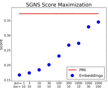
Figure 1: SGNS objective function score of trained embeddings models, compared to the optimal PMI-based score.dimanditerdenote the dimensionality and training iterations used for each model.
4 Experiments
In this section we useword2vecto train real skip-gram with negative sampling (SGNS) embedding models. By measuring the value of their objec-tive function and comparing it against the optimal one using exact PMI values, we demonstrate how a well-trained model minimizes the difference in Eq. (10). We note that this is an intrinsic measure that does not necessarily reflect the usefulness of the learned embeddings for other tasks.
We used the Penn Tree Bank (PTB), a popu-lar small-scale corpus, for our experiments. A version of this dataset is available from Tomas Mikolov.1 It consists of 929K training words with
a 10K word vocabulary, which we used to train our models. To learn the SGNS word embeddings, we used word2vec’s default parameter values: window-size = 5, min-count = 5, and number of negative samplesk = 5. We varied the dimensionality of
the embeddings and the number of training itera-tions performed. Once the models were trained, we measured their score (9) on the training corpus.
Based on the same learning corpus, we computed S(pmi) = JSMIα(X, Y) for α = k+11 = 1/6.
Note thatp(x, y) = 0implies that pmix,y=−∞
and thereforelogσ(−pmix,y) = 0. Hence, as in the second term, to compute the third term ofS(m)
(8) for the case of m = pmi, we can sum only
1http://www.fit.vutbr.cz/~imikolov/
over the positive pairs(x, y)that actually appear in the corpus.2 In other words, for the special
casem = pmi, it is feasible to compute the
ex-act score (8) and not just its approximation (9) that is based on negative sampling. Figure1illustrates the optimal PMI-based score, compared with the scores obtained by different models with varied embedding dimensionality and number of training iterations. As can be seen, the embeddings score gets close to the optimal value using higher dimen-sionality and more training iterations, but doesn’t surpass it.
5 Conclusion
In this study, we developed a new correlation mea-sure between random variables, denoted JSMI. This measure is based on the JS divergence and dif-fers from the standard mutual information measure that is based on the KL divergence. We showed that the optimization of skip-gram embeddings with negative sampling finds the best low-dimensional approximation of the JSMI measure. Thus, we pro-vided an information theory framework that hope-fully contributes to a better understanding of this embedding algorithm. Furthermore, although we focused here on the case of word-context joint dis-tributions, the connection we haven shown between the PMI matrix and the JSMI function is valid for every joint distribution of two random variables.
Acknowledgments
This work is supported by the Intel Collaborative Research Institute for Computational Intelligence (ICRI-CI).
References
Sanjeev Arora, Yuanzhi Li, Yingyu Liang, Tengyu Ma, and Andrej Risteski. 2016. A latent variable model approach to pmi-based word embeddings. Transac-tions of the Association for Computational Linguis-tics4:385–399.
Mohit Bansal, Kevin Gimpel, and Karen Livescu. 2014. Tailoring continuous word representations for depen-dency parsing. In Association for Computational Linguistics (ACL).
Carl Eckart and Gale Young. 1936. The approximation of one matrix by another of lower rank. Psychome-trika1:211–218.
2We used the exact same positive co-occurrence pairs
sam-pled by word2vec during the training of the SGNS embeddings to computeS(pmi).
Amir Globerson, Gal Chechik, Fernando Pereira, and Naftaly Tishby. 2007. Euclidean embedding of co-occurrence data. Journal of Machine Learning Re-search8:2265–2295.
Daniel D. Lee and H. Sebastian Seung. 2000. Algo-rithms for nonnegative matrix factorization. In Ad-vances in Neural Information Processing Systems.
Omer Levy and Yoav Goldberg. 2014. Neural word embedding as implicit matrix factorization. In Ad-vances in Neural Information Processing Systems.
Omer Levy, Yoav Goldberg, and Ido Dagan. 2015. Im-proving distributional similarity with lessons learned from word embeddings. Trans. of the Association for Computational Linguistics3:211–225.
Jianhua Lin. 1991. Divergence measures based on the shannon entropy. IEEE Transactions on Information Theory37(1):145–151.
Tomas Mikolov, Ilya Sutskever, Kai Chen, Greg Cor-rado, and Jeffrey Dean. 2013. Distributed represen-tations of words and phrases and their composition-ality. InAdvances in Neural Information Processing Systems.
Alexandre Passos, Vineet Kumar, and Andrew McCal-lum. 2014. Lexicon infused phrase embeddings for named entity resolution. InConference on Natural Language Learning (CoNLL).
Jeffrey Pennington, Richard Socher, and Christopher D Manning. 2014. Glove: Global vectors for word representation. InEMNLP. volume 14, pages 1532– 1543.
Karl Stratos, Michael Collins, and Daniel J Hsu. 2015. Model-based word embeddings from decomposi-tions of count matrices. In ACL (1). pages 1282– 1291.