Exam 1, Thursday January 8 (1) For each of the following transfer functions, determine if the system is asymptotically

ECE-520: Discrete-Time Control Systems Homework 3

Due: Tuesday January 6 in class Exam 1, Thursday January 8

1) For each of the following transfer functions, determine if the system is asymptotically stable, and if so, the estimated 2% settling time for the system. Assume the sampling interval is T =0.1 seconds.

a) 2

( 0.1) . ) (

( 0 2 )

H z

z z

z = +

− + d) 2

1 ( )

0.5 H z

z +z =

+

b) ( ) 1

( 2)( 0.5 H z

z z

=

− + ) e) 2

1 0.5 ( . ) 0 2 z H z

z + z+ − =

c) ( ) 1

( 0.1)( 0.5) H z

z z

=

− − f) 2

1 ( )

5 H z

z + +z =

Scambled Answers: 0.497, 0.58 , 1.15, 0.24, two unstable systems

2) For the following system, assuming the closed loop systems are stable, determine the prefilter gain G_pf that will result in zero steady state error for a unit step input. Are any of these systems type one systems?

a) ₂ 0.2 , ( ) , ( )

1 0.1 0.2

( )

p c

z

G z H z

z G z

z z

= =

−

+ + =1

b) ₂ 0.2 , ( ) , ( )

0.1 0.

1 ( )

2

p z G zc z

z

G H

z z

= =

+ + =1

c) ₂ , ( ) , ( ) 1

0.2 0.2

0.4 0

1 0.2

( )

.04

p G zc _z H z _z

z z

G z = =

+ +

3) Consider the continuous-time plant with transfer function 1

( )

( 1)( 2

p s _s

G

s =

)

+ +

We want to determine the discrete-time equivalent to this plant, , by assuming a zero order hold is placed before the continuous-time plant to convert the discrete-time control signal to a continuous time control signal.

( )

p G z

a) Show that if we assume a sampling interval of T , the equivalent discrete-time plant is

2 2

2

(0.5 0.5e ) (0.5 0.5 )

( )

( )( )

T T T T

p _{T T}

z e e e e

G z

z e z e

− − − − −

− −

− + + − +

=

− −

3T

Note that we have poles were we expect them to be, but we have introduced a zero in going from the continuous time system to the discrete-time system.

b) The Matlab script continuous_discrete_ft.m shows how to use Matlab to convert a discrete-time plant to a continuous-time plant, just as we have done by hand here. It also shows how to simulate and plot the two responses and the effect of a zero order hold on our system. Run this code and turn in your plot.

4) Prelab: In this (and the next) lab you will be using Matlab’s sisotool to simulate and implement discrete-time PI and PID controllers for your one degree of freedom systems. This prelab presents a brief review of Matlab’s sisotool (the 6.5.1 version) and some of the things you will need to know to apply this to our problem.

The file DT_PID.mdl is a Simulink model that implements a discrete-time PID

controller. It is somewhat unusual in that the plant is represented in state-variable form, but this is the usual form we will using in this class. The Simulink model looks like the following:

The file DT_PID_driver.m is the Matlab file that runs this code. We will be utilizing Matlab’s sisotool for determining the pole placement and the values of the gains.

Before we go on, we need to remember the following two things about discrete-time systems:

• For stability, all poles of the system must be within the unit circle. However, zeros can be outside of the unit circle.

The basic transfer function form of the components of a discrete-time PID controller are as follows:

Proportional (P) term : C z( )=K E zp ( )

Integral (I) term: ( ) ₁

1 1

i i

K K

C z

z− z

= =

− −

z

Derivative (D) term : 1 ( 1)

( ) (1 ) d

d

K z

C z K z

z

− −

= − =

PI Controller: To construct a PI controller, we add the P and I controllers together to get the overall transfer function:

( ) ( ) 1 1 p i i p

K K z K

K z

C z K

z z

p

+ −

= + =

− −

In sisotool this will be represented as

2

( ) (

( )

( 1) ( 1)

K z az K z a C z

z z z

)

+ +

= =

− −

In order to get the coefficients we need out of the sisotool format we equate coefficients to get:

,

p i p

K = −Ka K =K K−

PID Controller: To construct a PID controller, we add the P, I, and D controllers together to get the overall transfer function:

2 2 2

( 1) ( 1) ( ) ( 2 )

( 1) ( )

1 ( 1) ( 1)

p i d p i d p d

i d

p

K z z K z K z K K K z K K z K

K z K z

C z K

z z z z z z

− + − − + + + − − +

−

= + + = =

− − −

d

In sisotool this will be represented as

2

( )

( )

( 1) K z az b C z

z z

+ +

=

−

In order to get the coefficients we need out of the sisotool format we equate coefficients to get:

, 2 ,

d p d i p d

K =Kb K = −Ka− K K =K K− −K

Sisotool (Brief) Example

A) Run the Matlab program DT_PID_driver.m. This program is set up to read the data file bobs_1dof_205.mat, which is a continuous time state variable model for a one degree of freedom torsional system, and implement a P controller with gain 0.0116. It will put the value of the transfer function for your system, G zp( ), in your workspace.

• Type sisotool in the command window • Click close when the help window comes up

• Click on view → open loop bode to turn off the bode plot. (Whatever is checked will be shown, we only want to see the root locus.)

B) Loading the Transfer Function

• Click on file → import

• A window on the left will show you the transfer functions in your workspace, while the window in the right will let you choose the control system

configuration.

• We will usually be assigning to block G (the plant), so type your transfer function name next to G and then enter. You must hit enter or nothing will happen.

( )

p

G z

• Once you hit enter, you should be able to click on the OK at the bottom of the window. The window will then vanish.

• Once the transfer function has been entered, the root locus is displayed. Make sure the poles and zeros of your plant are where you think they should be.

C) Odds and Ends :

You may want to fix the root locus axes. To do this,

• Click Edit → Root Locus → Properties • Click on Limits

• Set the limits

You may also want to put on a grid, as another method of checking your answers. Type Edit → Root Locus → Grid

D) Generating the Step Response

• Click on Analysis → Response to Step Command

• You will probably have two curves on your step response plot. To just get the output, type Analysis → Other Loop Responses. If you only want the output, then only r to y is checked, and then click OK. However, sometimes you will also want the r to u output, since it shows the control effort for P, I, and PI controllers. • You can move the location of the pole in the root locus plot and see how the step

response changes.

• The bottom of the root locus window will show you the closed loop poles corresponding to the cursor location. However, if you need all of the closed loop poles you have to look at all of the branches.

E) Entering a Compensator (Controller). We will implement a PI controller here

• Type Compensators → Edit → C

• Click on Add Real Zero or Add Real Pole to enter real poles and zeros. You will be able to changes these values very easily later. Since we want a PI controller, we need a pole to be a 1 and we need to be able to change the value of the zero. For now assume the zero is at -1.

• Click OK to exit this window.

• Look at the form of C to be sure it's what you intended, and then look at the root locus with the compensator.

• You can again see how the step response changes with the compensator by moving the locations of the zero (grab the pink dot and slide it) and moving the gain of the system (grab the squares and drag them). Remember we need all poles and zeros to be inside the unit circle for stability!

• Move the pole an zero around until the zero is approximately -0.295 and the gain is approximately 0.0563.

F) Printing/Saving the Figures:

To save a figure sisotool has created, click File → Print to Figure. Print out this figure and attach it to the homework.

G) Back to Matlab.

• Determine the correct values of a and K

• Enter these in the Matlab code DT_PID_driver.m

• Modify DT_PID_driver.m to compute the proportional and integral gains • Run DT_PID_driver.m and print out the picture and attach it to this homework.

H) Now your one degree of freedom system

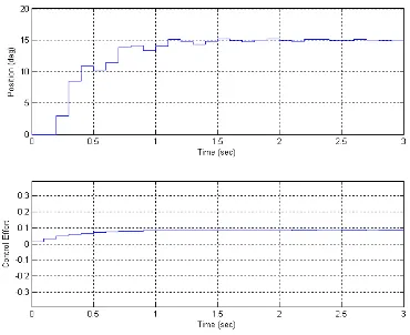
Choose one of your one degree of freedom systems (if there are two partners, each should choose a different system) and use a sampling interval of 0.1 seconds. For torsional (model 205) systems, assume a 15 degree step, for rectilinear (model 210) systems assume a 1 cm step. Use sisotool to determine a PI controller so you system has a settling time less than 1.5 seconds and a percent overshoot less than 25%. The control effort must also be within the allowed bounds, though this may be different than that output by sisotool since sisotool always assumes a step of value 1.

• Print out the root locus plot

• Determine the step response using sisotool and print out the graph

• Determine the step response using DT_PID_driver.m and print out the graph • Use sisotool to determine a PID controller so you system has a settling time less

than 1.75 seconds and a percent overshoot less than 25%. The control effort must also be within the allowed bounds.

• Print out the root locus plot

• Determine the step response using sisotool and print out the graph