1 ECE-320: Linear Control Systems
Homework 6
Due: Monday April 25 at the beginning of class
1) Consider a system with closed loop transfer function o( ) p p k G s
s k
. The nominal values for the
parameters are kp 1 and 2.
a) Determine an expression for the sensitivity of the closed loop system to variations in kp. Your final answer should be written as numbers and the complex variable s.
b) Determine an expression for the sensitivity of the closed loop system to variations in. Your final answer should be written as numbers and the complex variable s.
c) Determine expressions for the magnitude of the sensitivity functions in terms of frequency, d) As the system is more sensitive to which of the two parameters?
2) Consider the plant
0
1 3 ( )
0.5 p
G s
s s
where 3 is the nominal value of 0 and 0.5 is the nominal value of1. In this problem we will investigate the sensitivity of closed loop systems with various types of controllers to these two parameters. We will assume we want the settling time of our system to be 0.5 seconds and the steady state error for a unit step input to be less than 0.1.
a) (ITAE Model Matching) Since this is a first order system, we will use the first order ITAE model, ( ) o
o
o G s
s
i) For what value of owill we meet the settling time requirements and the steady state error requirements?
ii) Determine the corresponding controllerG sc( ).
iii) Show that the closed loop transfer function (using the parameterized form of G sp( ) and the controller from part ii) is
0
1 0
8
( 0.5) 3
( )
8
( ) ( 0.5)
3 o
s G s
s s s
iv) Show that the sensitivity of G so( )to variations in 0 is given by 0
0 8
G s
S s
2 v) Show that the sensitivity of G so( )to variations in 1 is given by 1 2
0.5 8.5 4 o G s S s s
b) (Proportional Control) Consider a proportional controller, with kp 2.5.
i) Show that the closed loop transfer function is 0
1 0 2.5 ( ) 2.5 o G s s
ii) Show that the sensitivity of G so( )to variations in 0 is given by 0 0 0.5 8 G s S s
iii) Show that the sensitivity of G so( )to variations in 1 is given by
1 0.5 8 o G S s
c) (Proportional+Integral Control) Consider a PI controller with kp 4 and ki 40.
i) Show that the closed loop transfer function is 0
1 0
4 ( 10) ( )
( ) 4 ( 10) o
s G s
s s s
ii) Show that the sensitivity of G so( )to variations in 0 is given by 0
0 2
( 0.5) 12.5 120
G s s
S
s s
iii) Show that the sensitivity of G so( )to variations in 1 is given by
1 2 0.5 12.5 120 o G s S s s
d) Using Matlab, simulate the unit step response of each type of controller. Plot all responses on one graph. Use different line types and a legend. Turn in your plot and code. Do not make separate graphs for each system!
e) Using Matlab and subplot, plot the sensitivity to 0 for each type of controller on one graph at the top of the page, and the sensitivity to 1 on one graph on the bottom of the page. Be sure to use different line types and a legend. Turn in your plot and code. Only plot up to about 8 Hz (50 rad/sec) using a semilog scale with the sensitivity in dB (see next page). Do not make separate graphs for each system!
In particular, these results should show you that the model matching method, which essentially tries and cancel the plant, are generally more sensitive to getting the plant parameters correct than the PI
controller for low frequencies. However, for higher frequencies the methods are all about the same.
Hint: If ( ) 2 2 2 10
s T s
s s
, plot the magnitude of the frequency response using:
T = tf([2 0],[1 2 10]); w = logspace(-1,1.7,1000); [M,P]= bode(T,w);
3
xlabel('Frequency (rad/sec)'); ylabel('dB');
3) Assume x t( ) 3 2cos(2t3) is the input to an LTI system with transfer function
2
2 | | 3
( )
3 | | 3
j
j
e H j
e
The steady state output will be
a) y t( ) 6 4cos(2t5) b) y t( )4cos(2t5) c) ( )y t [3 2cos(2t3)][2ej]
d) y t( ) 6 4cos(2t3)ej2 e)y t( ) 3 4cos(2t5) f) none of these
4) Assume ( ) 2 sin(5 ) 3cos(8 30 )o
x t t t is the input to an LTI system with transfer function shown below
The steady state output of this system will be
a) ( )y t 20 5sin(5 t90o) 6cos(8 t90 )o b) ( )y t 2 5sin(5t90 ) 6cos(8o t90 )o
c) ( ) 20 5sin(5 90 ) 6cos(8o 120 )o
y t t t d) ( ) 10 5sin(5 90 ) 6cos(8o 120 )o
y t t t
4 Problems 5 and 6 refer to a system whose frequency response is represented by the Bode plot below
.
5) If the input to the system is x t( )5cos(10t30o), then the steady state output is best estimated as
a) yss( )t 0 b) ( ) 5cos(10 30 ) o ss
y t t
c) yss(t)5cos(10t20 )o d) yss(t)5cos(10t50 )o
6) If the input to the system is x t( )50si (10n 0 )t , then the steady state output is best estimated as
a) yss( )t 2000sin(100t100 )o b) ( ) 0.5sin(100 100 ) o ss
y t t
c) ( ) 2000sin(100 100 )o ss
y t t d) ( ) 5sin(100 100 )o ss
y t t
100 101 102
-40 -30 -20 -10 0 10 20
M
a
g
n
it
u
d
e
(
d
B
)
Frequency (rad/sec)
100 101 102
-150 -100 -50 0 50
P
h
a
s
e
(
d
e
g
)
5 7) For the straight line approximation to the magnitude portion of a Bode plot shown below, the best estimate of the corresponding transfer function is
a)
1
20 1
0 )
1
( 10
1
H
s s
s
b)
1
10 1
0 )
1
( 10
1
H
s s
s
c) 2
1
10 1
10 (
(1 1) )
0
H
s s
s
d)
2
2 1
10 1
10 (1 ( )
0 1) H
s s
s
10-2 10-1 100 101 102
-80 -60 -40 -20 0 20 40 60
M
a
g
n
it
u
d
e
(
d
B
)
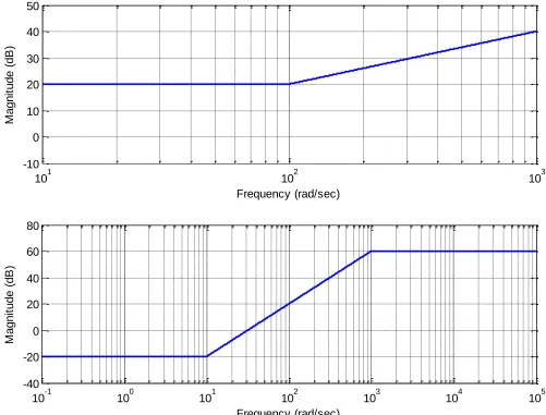
6 8) For the straight line approximation to the magnitude portion of a Bode plot shown below, the best estimate of the corresponding transfer function is
a) 2 1 1 100 0.01 ( ) 1 1 10 H s s s
b)
2 1 40 1 100 ( 1 1 10 ) s s s H c) 3 1 0.01 1 100 1 ) 1 10 ( H s s s
d) 2
3 1 0.01 1 100 1 1 ) 1 ( 0 H s s s
100 101 102 103 104
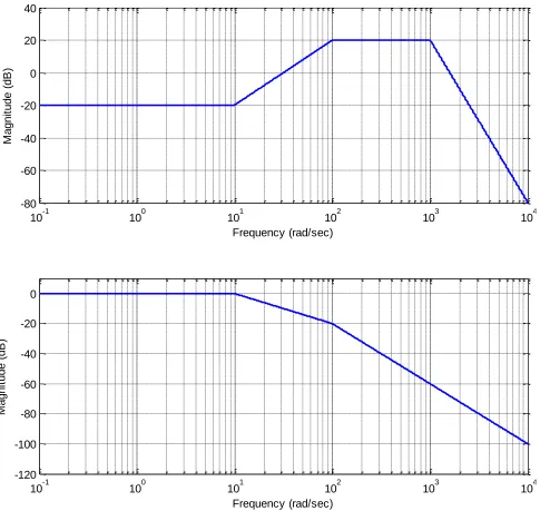
7 9) The following three figures display the magnitude of six transfer functions. All of the poles and zeros of these transfer functions are in the left half plane (these are minimum phase transfer functions). All of the magnitudes, poles, and zeros are either zero or simple powers of 10 ( etc). Estimate the transfer functions.
Figure 1: Problem 9,Systems a and b
1 1 2
10 ,1,10 ,10
100 101 102 103
-100 -50 0 50 100
M
a
g
n
it
u
d
e
(
d
B
)
Frequency (rad/sec)
100 101 102 103
-120 -100 -80 -60 -40 -20 0
M
a
g
n
it
u
d
e
(
d
B
)
8 Figure 2: Problem 9,Systems c and d
101 102 103
-10 0 10 20 30 40 50
M
a
g
n
it
u
d
e
(
d
B
)
Frequency (rad/sec)
10-1 100 101 102 103 104 105
-40 -20 0 20 40 60 80
M
a
g
n
it
u
d
e
(
d
B
)
9 Figure 3: Problem 9,Systems e and f
10-1 100 101 102 103 104
-80 -60 -40 -20 0 20 40
M
a
g
n
it
u
d
e
(
d
B
)
Frequency (rad/sec)
10-1 100 101 102 103 104
-120 -100 -80 -60 -40 -20 0
M
a
g
n
it
u
d
e
(
d
B
)
1 0
Answers:
10) (We will be using this in lab 5!, You mostly just run code for this problem) Assume we have reason to believe that the plant we want to design a controller for has the form
2
2 2
( )
2 p
n n
G s Ks
s s
and we need to estimate the paramters K, , and n.
Since we get transfer functions from LTI systems, one way to estimate these parameters is to experimentally construct a Bode plot of the system by using inputs of known frequencies and
amplitudes, and then measuring the amplitude and time delay (phase shift) of the output. Once we have the data for a Bode plot, we try and optimize the transfer function parameters to provide the best fit to the data. If this brings back nightmares of the last two labs in ECE205, then that class was not a complete waste of your time.
The Matlab program process_data_pendulum.m (from the class webpage) has some data collected for you for an experiment I did with the pendulum systems. Yout will be filling in the data for this program when you have your own system in the next lab. The first column is the input the frequency (in Hz), the second column is the input amplitude (0.087, in rad), the final column is the average output amplitude (in rad). Note that here we will only be estimating the magnitude portion of the Bode plot, so we are not concerned with the time delay (or phase change) between the intput and output.
In the Matlab command window, type data = process_data_pendulum
This will write to the array data, and write the frequency and gain at that frequency to the screen. Remember the frequency at which the maximum gain occurs.
To estimate the parameters we need we will use the Matlab program model_pendulum.m (from the class website)which utilizes Matlab’s fminsearch routine. The input arguments to
2
2 2
2 2
2 2 5
1
0.1 1
100 100 1
, ( ) , ( ) 10 1
100
1 1
0.1 1 0.1 1
1
10 10
, ( )
1 1
1 1 1 1 1
1 1 1
10 100
1000 100 1
(
0 )
( , )
00
) (
H s
H s H
s
H s H s s
s s
s s
H s
s s
s s s
s
1 1 model_pendulum.m are the array data, the initial guess of the parameter K (assume it is 1.0), the initial guess of the parameter