EC 300 Signals and Systems Spring 2007
S
YSTEML
INEARITYLab 3
Mario F. Simoni and Robert Throne
Prelab:
Obtain the necessary components as listed below from the parts room, C117, and wire up the circuit on your breadboard before coming to lab.
Objectives
The purpose of this lab is to gain a better understanding of what LINEARITY means in reference to a real system. You will begin the lab by building a transistor amplifier circuit and measuring the input and output signals as you vary the amplitude of your input signal. You will then compare the results of your experiment to the “expected” outputs by plotting your results in Matlab.
This lab will use the following components:
1-100 uF electrolitic capacitor 1-Q2N3904 NPN BJT transistor
Resistors (1 ea.) – 1K, 1.2K, 9.1K, 10K, 51K, and 300K
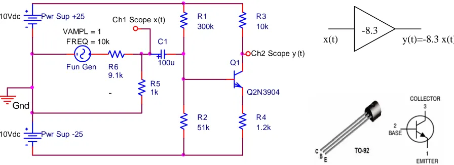
Build the common-emitter amplifer, shown in Figure 1 below, on your breadboard before coming to lab. The pins for the transistor are shown next to the circuit diagram.
Q1 Q2N3904 R1 300k R2 51k R3 10k Pwr Sup +25
10Vdc
Pwr Sup -25
10Vdc
Fun Gen
FREQ = 10k VAMPL = 1
Gnd
R4 1.2k
Ch2 Scope y (t)
R5 1k R6 9.1k C1 100u
Ch1 Scope x(t)
x(t) -8.3 y(t)=-8.3 x(t)
[image:1.612.78.526.444.607.2]-
Figure 1: Circuit Diagram of the common-emitter amplifier. The pin layout for the transistor is shown to the right. The ideal block diagram representation for this amplifier is shown as the triangle in the upper right.
the nonlinearities of the transistors begin to affect the signal. When the input signal to the amplifier is “small”, we can approximate the transistor with its small-signal model that is composed of linear elements. As long as the input signal stays small, the amplifier behaves like an ideal device. However, when the input to the amplifier is “large”, the nonlinearities of the amplifier can be observed, and we have to use the large-signal model (exponential for BJT, square-law for FETs) of the transistor to understand the operation of the amplifier. “Large” and “small” are fuzzy terms and, as system designers, we would like to have a more quantitative definition for these values. With respect to the amplitude of the input signal, the amplifier’s nonlinearities decrease the gain, called gain compression, and distort the shape of the output signal, called harmonic distortion. One way to quantitatively define “small” versus “large” signal is to measure the magnitude of the input voltage at which the gain begins to decrease, called the compression point. Another is to define an acceptable level of distortion and the amplitude threshold at which this distortion level occurs. You won’t understand how to measure the distortion in the signal until the end of this quarter. This lab will focus on measuring the gain compression point while simply observing the distortion that occurs in the output due to the nonlinearities of the amplifier. The goal of the first part of this lab is to:
1. Measure the gain compression point for the amplifier
2. Record the output of the amplifier on the oscilloscope for both a “large” and “small” signal input to observe the distortion.
a) Build the amplifier as shown in the figure above. Hook up the power supplies and the function generator. Hook up the oscilloscope probes to the nodes labeled x(t) (the input to the amplifier) and y(t) (the output of the amplifier). Of special note when assembling and testing the amplifier:
1. Make sure the capacitor’s positive node is connected as shown in the figure above.
2. The DC Bias points (node voltages relative to Gnd measured with the DMM set to DC Volts) of the amplifier should be approximately: VBase=-7.4 V, VCollector=-5.4 V, and
VEmitter=-8.1 V
3. Make sure you connect your power supplies with the right polarities.
4. The voltage divider connected to the function generator reduces the amplitude of the function generator by a factor of approximately 10. When doing your experiments, make sure you measure the input to the amplifier (on the positive node of the capacitor) not the output of the function generator.
5. Set the coupling of the oscilloscope to AC and the probe gains to 10:1 for each channel. Do not use autoscale because it will change your coupling back to DC.
6. Use the Acquire button on the oscilloscope to automatically measure the peak-peak voltages of both signals.
Instructor Verification (see last page)
b) Set the function generator to be a sinusoid with frequency of 10 kHz. Start with the peak-peak amplitude of x(t)=50 mV. Measure the peak-peak voltage of both x(t) and y(t) as you sweep the amplitude of x(t) from 50mV to 490mV in 20mV increments (a total of 23 data points). NOTE: The the peak-peak amplitude of x(t) is different from the function generator because of the voltage divider. You will need to sweep the function generator’s peak-peak amplitude from
approximately 500mV to 4.9V in 200mV increments. Record your data in the table at the end of this handout and then enter the vectors into a Matlab m-file.
c) In the same m-file, plot the gain of the amplifier (vout/vin) for each input voltage amplitude. Your plot should look like the following figure. Include in your plot a line that indicates the ideal gain of your amplifier. The ideal gain can be found by averaging the measured gain for the first few “small-signal” data points.
d) You can get a rough estimate of the gain compression point by looking at your plot. This point is defined as the input voltage at which the gain begins to decrease and is indicated by the red circle in the figure above. You should indicate your gain compression point similarly in your plot. Use the menu commands in the figure window to insert an ellipse.
e) In the same m-file, use the polyfit command in Matlab to fit a line to only the data below the gain compression point using x(t) as your x-coordinates and y(t) as your y-coordinates for the polyfit command.
Instructor Verification (see last page)
g) Now that you’ve found the gain compression point, you can quantitatively define “small” and “large” signal. Record a screen capture from the oscilloscope showing the output traces for the input and output voltages for both a “small-signal” value of x(t) and a “large-signal” value of x(t). Print out these screen captures to hand in with your lab. Indicate on the printouts where the nonlinearities of the amplifier cause distortion.
i) Also hand in your table with the recorded data files and the final m-file that includes your code for data analysis
Report
For this lab, turn in all of your Matlab code and plots in addition to this verification sheet.
Lab 03 System Linearity Instructor Verification Sheet
Name ___________________________________________ Date of Lab: __________________
Part (a) Demonstrate that your circuit works appropriately.
Verified: _________________________________________ Date/Time: __________________
Part (f) Present your plots.
Verified: _________________________________________ Date/Time: __________________
Part (i) Present your plots.
x(t) (mVp-p) y(t) (mVp-p)
50
70
90
110
130
150
170
190
210
230
250
270
290
310
330
350
370
390
410
430
450
470