EZ10335
REVIEW COPY
NOT FOR DISTRIBUTION
Self-consistent analytic solution for the current and the access
resistance
in open ion channels
D. G. Luchinsky1,4, R. Tindjong1, I. Kaufman2,
P.V.E. McClintock1, R.S. Eisenberg3
1Department of Physics, Lancaster University, Lancaster LA1 4YB, UK.
2 VNII for Metrological Service, Gosstandart, Moscow, 119361, Russia.
3Department of Molecular Biophysics and Physiology, Rush Medical college,
1750 West Harrison, Chicago, IL 60612, USA. and
4Mission Critical Technologies Inc.,
2041 Rosecrans Ave. Suite 225 El Segundo, CA 90245
Abstract
A self-consistent analytic approach is introduced for estimation of the access resistance (AR) and current through an open ion channel for an arbitrary number of species. For an ion current flowing radially inwards from infinity to the channel mouth, the Poisson-Boltzmann-Nernst-Planck (PBNP) equations are solved analytically in the bulk with spherical symmetry in three dimen-sions (3D), by linearization. Within the channel, the Poisson-Nernst-Planck (PNP) equation is solved analytically in a one-dimensional (1D) approximation. An iterative procedure is used to match the two solutions together at the channel mouth in a self-consistent way. It is shown that the current-voltage characteristics obtained are in good quantitative agreement with experimental measurements.
PACS numbers: 66.10.-x, 87.16.Vy, 87.90.+y
Keywords: Ion channels, Poisson equation, Nernst-Planck equation, access resistance, self-consistent
I. INTRODUCTION
Ion channels are natural nanotubes in cellular membranes [1, 2], capable of conduct-ing up to 108 ions per second, selectively, through the membrane. They control a vast
range of biological functions. Understanding their properties from physical first principles is a long-standing fundamental scientific problem of great interdisciplinary importance, with numerous potential applications, including e.g. a fast growing area of research in nanoflu-ids [3]. Theoretical treatments of ion transport through channel proteins may be classified broadly as rate theoretical approaches [4], electro-diffusion models [5], stochastic models [6], or molecular dynamical models [7]. Of these, the first two have the advantage of providing analytic insight into the properties of ion channels over a wide range of parameters. For example, analytic approximations for the Poisson equation in the pore have been derived in [8–10]. Quasi-analytic estimations of the channel current voltage characteristics using Poisson-Nernst-Planck (PNP) theory became indispensable numerical tools in ion channel analysis because of their simplicity, physical clarity, and good quantitative agreement with experimental results [11–15]. At the same time, in most cases, the access resistance (AR) of the channel’s two apertures contributes between 10 and 30 % of the overall channel re-sistance [16] and there are channels for which the AR is believed to limit the channel’s conductivity [17].
full 3D set of PNP equations in the channel [24] and Poisson-Boltzmann (PB) equations in the bulk and in the channel [25]. Very interesting asymptotic results for access resistance problem of uncharged particles, where the mean time of absorbtion of a Brownian particle to a narrow window is calculated were obtained in [26]. The AR problem was considered in [13, 27, 28] where a modification of the Donnan potential formalism and the PNP model were used to obtain an approximation for the electrostatic potential at the interface between the channel and the surrounding ionic solution. This approximation is valid for channels longer than 20 ˚A, and requires a step-wise change of the excess chemical potential at the channel entrance as well as charge neutrality inside the channel.
Despite all this recent progress, an analytic solution able to connect in a self-consistent manner the ion currents and electrostatic potentials in the access resistance region in the bulk with those in the pore is still lacking. If available, such a solution would allow for simultaneous semi-analytic estimations of the AR and current in many real ion channels, providing further physical insight into their properties. It would also allow one to set up boundary conditions for the electric field and concentrations at the channel mouths in a self-consistent way. It is therefore very desirable to extend the theory by seeking self-self-consistent simultaneous solutions of the AR problem and PBNP in the bulk, and the PNP solution in the pore.
In this paper we present such an extension, combining both solutions by means of a simple, quasi-analytic, iterative procedure. The solution is continuous in concentration, electrostatic potential and electric field, and it satisfies Dirichlet boundary conditions for the concentration and potential in the bulk at plus and minus infinity. It is valid for any number of monovalent ion species and allows for simultaneous self-consistent estimations of the access resistance, potential and current for each species.
The system considered is made of three compartments (see Fig. 1). The main compart-ment is a cylindrical channel in the protein which allows ions to cross the membrane. The membrane is bathed by two solutions of different concentration on its left and right hand sides. The electro-diffusion in this system is described by the Poisson equation (in SI units)
∇ ·[ε(r)∇φ˜m(r)] =− N
X
i=1
combined with the continuity equations for mobile ions
∂n˜j(r, t)
∂t +∇ ·J˜j = 0, (j = 1, ..., N), ˜
Jj =−Dj(r)
∇n˜j+
˜ nj(r)
kBT ∇
˜ ψj
. (2)
Here ˜φm(r) is the average at a given location r in 3D space electrostatic potential due to
all mobile ions and applied electric field, ˜ψj is the ion free energy, and ˜nj(r) is the number
densities of mobile ions. ˜nj(r) = 103NAc˜j(r), where ˜cj(r) is the concentration (in mole/liter)
of mobile ion species j characterized by the the valence zj, the flux ˜Jj, and the diffusion
constant Dj. N is the number of species. The Nernst-Planck equation is the sum of fluxes
due to local gradients of concentration and potential. NA is Avogadro’s number. Other
parameters ε, e, kB, T are respectively the dielectric constant, the elementary charge, the
Boltzmann constant, and the temperature.
Ion free energy is conveniently divided into two contributions [29]
˜
ψj(r) = zjeφ˜m(r) + ˜ψjP M F(r), (3)
where ˜φm(r) satisfy the Poisson equation (1) and ˜ψP M Fj (r) is the part of the free energy
associated with the potential of the mean force in the channel [30] that depends on the ion size and can be responsible of for e.g. strong channel selectivity between alike ions [31]. In one of the obvious generalizations the ˜ψP M F
j (r) includes the electrostatic charge of the
protein walls [24, 29, 32], i.e. ˜ψP M F
j (r) =zjeφ˜p(r), where ˜φp(r) is the electrostatic potential
due to fixed charge on the protein walls. A less obvious contribution due to the finite size of the ions and molecules of water will be considered in details elsewhere. In the present consideration we will approximate the corresponding contribution to the free energy by a single parameter – filling factor – which is discussed in the following section.
We note that equations (1), (2) allow one to consider modulation of the ionic flux through the channel due to the e.g, wall vibration (cf [33]). In the standard approximation, however, the steady state (∂n˜j(r,t)
∂t = 0) solution of the PNP equations is of interest and we arrive to
the following set of equations
∇ ·[ε(r)∇φ˜(r)] =−
N
X
i=1
zjen˜j(r)−ep˜ex(r),
∇ ·
Dj(r)
∇n˜j +
zjen˜j(r)
kBT ∇
˜ φ
= 0,
FIG. 1: Geometry of the model system under consideration. It is comprised of a cylindrical pore and two hemisphere at the left- and right-hand mouths of the channel. The three different regions of the solution are marked as I – bulk, II – boundary hemispheres, and III – pore.
where ˜φ(r) = ˜φm(r) + ˜φp(r), and ˜pex(r) is the number density of the partial charges fixed
on the protein and lipid atoms.
The system of eqs. (4) is solved in the bulk in Boltzmann approximation in 3D assuming spherical symmetry (the PBPN solution in the regions I, Fig. 1) and in the pore in 1D approximation [8] (the PNP solution in the region III, Fig. 1). For the PBNP solution the boundary conditions (BC) for potential and concentration are set at ± infinity, while the BC for the current and gradient of the potential are set at the surfaces of two hemispheres of radius a. For the PNP solution the BC for potential and concentration are set directly at the channel entrances. In the boundary hemispheres (regions II, Fig. 1) a linear approx-imation (cf. [22]) is introduced in the hemispheres to ensure the continuity of the solutions. To obtain a simultaneous self-consistent solution in the bulk and in the pore a matching procedure is developed. Using this procedure the I −V characteristics are calculated for Gramicidin A (GA) channel and the results of calculations are compared with the exper-imental results obtained by two different groups. The access resistance found using this procedure is compared with the AR calculated from the Hall formula.
We demonstrate in Sec. IV that the boundary condition problem for solutions of the equa-tions inside and outside the channel can be resolved uniquely. The joint solution is then obtained in Sec. V and compared with experimental results. In Sec. VI we analyse channel properties by investigating the influences of membrane fixed charge and bulk concentration on the permeation process. Finally, in Section VII, we summarize and present conclusions.
II. SOLUTION OF THE PNP EQUATIONS IN THE CHANNEL
A. The 1D solution of the Poisson equation
Useful insight (see e.g. [12–15] and references therein) into the functions of many channels can be obtained from a one-dimensional approximation of equations (1), (2) within the channel, modeling it as a tube with cylindrical symmetry. Using results of [8, 9] the Poisson equation for a long, narrow channel can be written as
−εd
2φ˜
dx˜2 =zpep˜ex+e
N
X
j=1
zjn˜j + ˜ε
˜ ∆
1−x˜ d
−φ˜
, (5)
˜
φ(˜x0) = ˜φ0, φ˜(˜x1) = ˜φ1, Vapp= ˜φ1−φ˜0 = ˜∆.
This approximation is valid for any numberN of ionic species in the solution. For simplicity, the dielectric constant is taken to be independent of time and space. The first term on the right-hand side represents the linear density of permanent charge on the atoms of the protein, i.e. the charge that is independent of the electric field. The total wall charge zpe, and the parameters of the associated distribution of the permanent charge ˜pex(x), are
fitting parameters to be determined by comparison with experiment. The second term is the channel contents, consisting of free (mobile) charge, carried by ions in the pore as they move through the channel. The last term is the induced (i.e. polarization) charge on the protein walls of the pore [34]. The dielectric properties of the channel protein and its water-filled pore (radiusa, lengthd) are described by the permittivity of free space; the (dimensionless) dielectric constants of the protein εp and water εH2O and the effective dielectric constant of the channel [8, 9]
˜ ε≡ εp
εH2O
The constant ˜∆ is the potential difference across the channel, and parameterε=ε0εH2O. To solve Poisson’s equation we write it in dimensionless form using the following characteristic length and potential:
˜
φ=φUT, x˜=xd, UT =
kBT
e , ˜
pex = ˜n∞Lpex, ˜nj = ˜n∞Lnj.
(6)
The dimensionless number densities for the fixed and mobile charges are introduced by normalization of ˜pex and ˜nj as follows
Nf = ˜n∞LS
Z d
0
dx˜p˜ex(˜x)
˜ n∞
L
= ˜n∞
Lv0
Z 1
0
dxpex(x),
Nm = ˜n∞LSef f
Z d
0
dx˜˜nj(˜x)
˜ n∞
L
= ˜n∞
Lv0
Z 1
0
dxfscnj(x) (7)
where Nf and Nm are the number of elementary fixed and mobile charges, v0 = S ·d is
the pore volume, S and Sef f are actual and effective cross-sectional areas for the fixed and
mobile ions, and fsc is the filling factor defined as Sef f = fscS. In scaling equations (7)
the bulk concentration on the far left is used as the reference concentration. The physical meaning of the Sef f, is that because of their finite size and interaction with the wall, the
mobile ions can fill only an effective channel cross-section as will be explained in more details in Sec. II D.
The dimensionless Poisson equation has the form:
φ′′−η2φ=−η2∆(1−x)−zpα2p−α2 N
X
j=1
zjnj, (8)
φ(x0) =φ0, φ(x1) =φ1, ∆ =φ1−φ0.
Here we have introduced two dimensionless parameters, η and α, given by
η2 =d2ε/ε, α˜ 2 = d
2en˜∞
L
εUT
.
Note that (α/d)−1 is an effective Debye length in the channel.
φ(x) = (φ1−φ0) (x1−x0)
(x−x0) +φ0+
Z x1
x0
G(x, s)f(s)ds,
f(s) =η2
(φ1−φ0)
(x1−x0)
(s−x0) +φ0−∆(1−s)
−α2zpp(s)−α2 N
X
j=1
zjnj(s),
G(x, s) =
Asinhη(s−x1) sinhη(x−x0), x0 ≤x≤s.
Asinhη(s−x0) sinhη(x−x1), s≤x≤x1.
(9)
Here, G(x, s) is the associated Green’s function and A= 1/(ηsinhη(x1−x0)). The
perma-nent charge is modeled using a uni- or multi-modal Gaussian distribution, consistent with the fact that it is induced by local charges on the channel wall [35, 36]:
p(x) =
M
X
i=1
1
p
2πσ2
i
exp
−(x−µi)
2
2σ2
i
, (10)
whereµi andσi are the mean value and the variance of the coordinate of the ith wall charge.
The parameters of this distribution, together with the parameters of the axial distribution of the diffusion coefficient for each ion species, are the fitting parameters of the model. Having estimated the solution of Poisson’s equation, we now focus on the Nernst-Planck equation for determination of the current density and concentrations of the two ion species.
B. Solution of the Nernst-Planck equation in the channel
The problem to be discussed in this subsection is one described by Eisenberg et al [37]. The local concentration of ions of species j located on the axis between ˜x0 = 0 and ˜x1 =d,
satisfies the Nernst-Planck equation in the Stratonovich form [38]
d dx˜Dj
dn˜j(˜x)
dx˜ + zje
kBT
˜ nj(˜x)
dφ˜ dx˜
= 0 (11)
for ˜x0 ≤x˜≤x˜1,
which is the 1D form of Eq. (2). The diffusion coefficient Dj(˜x) is taken to be a function of
the position of the ion on the channel axis. Taking into account the normalization conditions (7), and the corresponding scaling for the effective cross-sectional area, the concentrations at the channel mouth result in the following boundary conditions for Eq. (11):
˜
Integrating Eq. (11) once, we obtain:
˜
Jj =−Dj
dn˜j(˜x)
dx˜ + zje
kBT
˜ nj(˜x)
dφ˜ dx˜
, (13)
where ˜Jj is the current density carried by ionsj (i.e. the current per unit area,
correspond-ing to the flux of ions j through the channel). We now rewrite this equation in terms of dimensionless variables. Using the scaling factors from Eqs. (6)–(7), the dimensionless Nernst-Planck equation is therefore given by:
Jjch = J˜jd Dj˜n∞L
=−
dnj(x)
dx +nj(x) dzjφ
dx
, (14)
nj(x=x0) =njL, nj(x=x1) =njR.
Integrating Eqs. (14), the analytic flux and concentration can [37] be calculated as
Jch
j =
njLezjφ0 −njRezjφ1
Rx1
x0 e
zjφ(s)ds , (15)
nj(x) =e−zjφ(x)
njLezjφ0 −Jjch
Z x
x0
ezjφ(s)ds
. (16)
Solution of the Poisson equation and the current density coupled to the ionic concentrations may now be calculated simultaneously in a self-consistent manner. The fitting parameters are the diffusion coefficient Dj together with the parameters describing the distribution of
fixed charge on the channel walls. The ionic currents ˜Jj inside the channel, and the total
current, are given by:
˜
Ij = zjeSef fJ˜j =
zjeDjn˜∞LSef f
d J
ch j , I˜=
N
X
j=1
˜
Ij. (17)
C. Self-consistent solution of Poisson-Nernst-Plank (PNP) equations in the chan-nel
A self-consistent (simultaneous) solution of the PNP equations (8) and (14) can be ob-tained using the well known Gummel [39] iterative procedure from semiconductor physics, ensuring that Poisson’s equation and the far-field boundary conditions are always satis-fied [2]. As a first step we calculate the concentrations making a linear initial guess for the potential
φ(x; initial guess) = (φ1−φ0) (x1−x0)
−300−2 −200 −100 0 100 200 300 −1
0 1 2
I (pA)
V (mV)
(a)
−300−2 −200 −100 0 100 200 300 0
2 4 6 8
I (pA)
V (mV) (b)
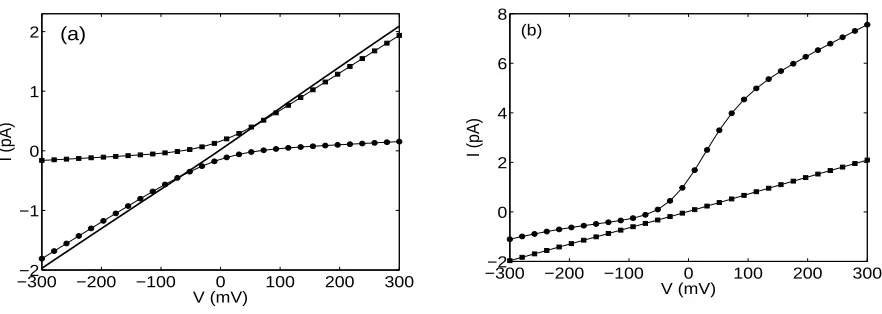
FIG. 2: (a) Calculated current-voltage (I−V) characteristics for the uncharged Gramicidin A (GA) channel. The thick line shows the total current, the squares represent positive ion current, and the filled circles represent negative ion current. The thinner lines joining calculated points are guides to the eye. Ionic concentrations in the lower (or left) and upper (or right) reservoirs arecL= 500 mM
and cR= 40 mM, respectively. Diffusion constants are D+=D− = 1.27×10⁻¹⁰ m2/s. To fit the result, we used a channel of radius = 4 ˚A, length = 30 ˚A with a filling factor of 0.16. (b) the corresponding current-voltage characteristics for charged GA (circles) with a filling factor of 0.28 and uncharged GA (squares).
Using the given concentrations and electrostatic potential in the bulk, we then set boundary conditions directly at the channel boundaries. Next we obtain concentrations and currents using Eqs. (15)-(17). The concentrations obtained are used to update the value of the potential. This procedure can be repeated to obtain higher order accuracy of the solution. Note that the linear part of the potential φ(x) in (9), the Green’s function (9), and the two first terms in the function (9) are fixed and have to be calculated only once during the iterations. This numerical procedure was used earlier by Eisenberg [40]. The difference in the present calculation is that we solve Poisson’s equation analytically and then couple it to the solution of the access resistance equations (see below).
The output of these calculations is the axial distributions of the electrostatic potential ˜
φ(x) and of the ions ˜cj(x), the current ˜Ij for species j, and the total current ˜I as a function
of the applied voltage and ionic concentrations in the bulk solutions.
[image:10.612.82.523.77.234.2]the I −V characteristic is linear. The effect of a net charge on the current is analyzed in Fig. 2(b) where we compare theI−V characteristic for an uncharged and a charged channel. The net negative wall charge used for this calculation is equal to−0.2e. It is distributed on the membrane walls using a two-mode Gaussian distribution with mean values µj equal to
1/6 near the channel mouth and 1/2 at the center of the channel. The variance is chosen as σ = 0.1. The results shown in the Fig. 2(b) are obtained with the same values of parameters for the channel geometry, diffusion coefficients, and concentrations as in [24] and are in good qualitative agreement with both the results of full 3D solutions of the PNP equations and with experimental measurements as compared to Figs. 5 and 6 of [24]. These results demonstrate that a simple calibration of the analytic solution allows one to get the same result as yielded by the full 3D simulations.
D. Filling factor
We note that the current in the I −V characteristics shown in Fig. 2 is calculated as I = eJ S˜ ch, where ˜J is the current density obtained using the self-consistent solution of
the PNP equations and Sch is the channel’s cross-sectional area. We note further that the
continuous approximation introduced above is valid only on the channel axis. Away from the channel axis the current density has to decay rapidly for a number of reasons. First, the ions that carry the current cannot come closer then their own radii to the channel wall. Secondly, the effective channel radius is further reduced due to the presence of dielectric walls of low dielectric constant. Indeed, the charges induced by an ion on the dielectric walls force the ion to stay near the channel axis, so that the probability of finding the ion at a finite distance r from the axis decays rapidly with increasing r. Moreover, the actual geometry of the channel is complicated (e.g. the channel is not cylindrical) and the channel can only be characterized by an effective radius averaged over the channel length. For these reasons, calculation of the total current through the channel using the axial current density ˜Jrequires one to introduce an effective cross-sectional area of the channelSch=Sef f =πa2fsc =πa2ef f
(see also [41]).
introduced as a simple approximation of the free energy contribution due to the potential of the mean force in the channel. We note also that factors of this type are common in semicon-ductor theories (cf. the ideality factor in the diode equation [42]) used to model conduction in ion channels [33]. The adjustment of the effective cross-sectional area of the channel in an analytic 1D approximation allows one to obtain qualitatively good agreement with the full 3D PNP solution of Kurnikova [24], whose results fit experiments. Therefore, taking into account earlier examples of the successful application of the 1D approximation (see e.g. [11–15]) our analytic solution can be calibrated with a suitably chosen filling factor and then used as a convenient tool for obtaining simple analytic estimates of the fundamental conducting properties of many ion channels.
The 1D approximation obtained above can be further improved by taking into account changes of the potential and the ion concentrations in the bulk. The latter difference can be estimated using e.g. the Donnan potential or access resistance formalisms as discussed in the introduction. In what follows we solve the problem using the access resistance formalism by coupling the PNP solution in the channel (discussed in this section) to the analytic solution of the PBNP equations in the bulk (next section) in a self-consistent manner.
III. SOLUTION OF THE PBNP EQUATIONS IN THE BULK
To find an analytic solution of the PBNP equations in the bulk in spherical symmetry, we follow closely the considerations of Peskoff [21]. As already mentioned, the solution in bulk spans from±∞ to a hemisphere at each channel mouth of radius equal to the effective radius of the channel.
A. Nernst-Planck equation in spherical symmetry
Consider first a solution of the Nernst-Planck equation (2), rewriting it in spherical symmetry as
˜
Jj =−Db,j
dn˜j(˜r)
d˜r + zje
kBT
˜ nj(˜r)
dφ˜ dr˜
, (19)
and setting the following boundary conditions at infinity
˜
and at the surface of the semi-sphere closed to the channel mouth
˜
Jj(˜r =aef f) = ±
˜ Ij
2eπa2
ef f
. (21)
Hereaef f is the effective radius of the channel, ˜Ij is the current of the jth ion found in the
solution of the PNP equations above inside the channel. The “−” sign is for ions in the left-hand bath and the “ + ” sign is for ions in the right-hand bath. We use the following scaling factors for the electric potential, the radial coordinate and the ion concentration:
˜
φ=φUT, r˜=rd, n˜j =njn˜∞L. (22)
The dimensionless form of Eq. (19) can then be written as
Jj =
˜ Jjd
Db,jn˜∞L
=−
dnj(r)
dr +nj(˜r) dzjφ
dr
, (23)
Integration of Eq. (19) with the boundary conditions (20) and (21) can be performed in a way similar to integration of (14), taking into account that ˜Jj(˜r) =±
˜
Ij
2eπr˜2. We thus obtain
nj(r) =
n˜∞
j
˜ n∞
L
ezjφ∞
∓βj
Z ∞
r
dse
zjφ(s)
s2
e−zjφ(r), (24)
βj =
˜ Ij
2eπn˜∞
LDb,jd
=aef f d
2 D
j
2Db,j
Jch
j . (25)
This solution can be further simplified if we neglect the change of potential in the bulk to obtain
nj(r) =n∞j ∓
βj
r . (26)
Note the difference in sign of this solutions arising from the difference in the radial directions in the left and right sections of the system (see Fig. 1).
B. Poisson-Boltzmann equation in spherical symmetry
The solution (24) depends on the electrostatic potential ˜φ(˜r), which can in turn be deter-mined by solution of the Poisson-Boltzmann equation. In spherical coordinates, for N ion species, this can be written as
ε1 ˜ r
d2
dr˜2(˜rφ˜) =−e
N
X
j=1
˜
φ(˜r=∞) = ˜φ∞
L, ∇φ˜(˜r=a) =∇φ˜P N P(˜x= ˜x0). (28)
whereε=εH2Oε0 is the product of the water dielectric constant and the electric permittivity of the vacuum, and ˜φP N P is the PNP solution obtained inside the channel as calculated in
Sec. II. At infinity, away from the channel mouth, the solution is assumed to be charge neutral (PN
j=1zj˜n∞j = 0). Note, however, that neutrality is not required at the channel
mouth, unlike in the Donnan potential formalism [27]. Using the dimensionless variables defined in Eq. (8), and substituting solution of the Nernst-Planck equation (23) into (27), we obtain the following integro-differential equation for monovalent ion solutions:
1 2α2r
d2
dr2(rφ) = sinh(φ(r)−φ
∞
L) +
1 2
X
j
zjn∞j βje−zjφ(r)
Z ∞
r
ezjφ(s)
s2 ds. (29)
We have assumed for simplicity that the diffusion coefficients do not depend of r, although this simplification can be readily lifted if necessary. The solution of the integro-differential equation is not trivial. It can be solved numerically to determine the electrostatic potential. However, it was shown by Peskoff [21] that the solution found in a linear approximation of the PB equation agrees well with the exact solution under most physiological conditions. Therefore, we linearize the PB equation for small values of the electrostatic potential and obtain reduced equation in the form [21]
1 2α2r
d2
dr2(rφ) = φ(r)−φ
∞
L +
β
r, (30)
whereβ = 1 2
P
jzjβj. Integration of Eq. (30) yields the following expression for the
electro-static potential:
φ(r) = (β+S0)e √
2α(aef f/d−r) 1 +√2αaef f/d
r − β
r +φ ∞
L, (31)
whereS0 = (aef f/d)2∇φP N P(x0) is proportional to the gradient of the electrostatic potential
Similarly, the bulk solution for the electrostatic potential on the right hand side can be written by making sure that the sign of the current density Eq. (21) is properly chosen
φ(r) =−(βf +S1)e √2n
fα(aef f/d−r) 1 +p
2nfαaef f/d
r +
βf
r +φ ∞
R. (32)
where S1 = (aef f/d)2∇φP N P(x1), nf = ˜n ∞
R ˜
n∞
L, and βf = 1 2nf
P
jzjβj. The factor nf appears
because we scale concentrations on both sides of the channel by the same value ˜n∞
L.
Eqs. (24), (31) and (32) provide the required solution of the PBNP equations in the bulk. To determine spatial distributions of the concentrationsnj(r) and the electrostatic potential
φ(r) (and their values at the channel mouth) in a self-consistent manner, these equations can be solved simultaneously using an iterative procedure analogous to that introduced in the previous section for the PNP solution.
Note that these solutions depend on the concentrations and electrostatic potential at infinity, the dimensionless current densities βj, and the gradient of electrostatic potential
∇φP N P at both mouths of the channel. The latter values are provided by the PNP solution in
0 10 20 30 40 50 60 70 80 90 −0.3
−0.25 −0.2 −0.15 −0.1 −0.05 0
φ
(V)
PB PNP PB
[image:15.612.201.408.387.532.2]x (˚A)
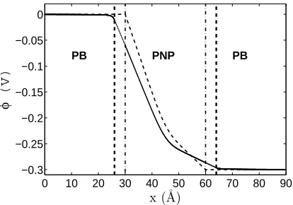
FIG. 3: Electrostatic potential in the model, calculated for the following boundary conditions:
φ(−∞) = φ∞
L = 0; φ(∞) = φ∞R = -300 mV; c(−∞) = c∞L = 500 mM; c(∞) = c∞R = 40 mM;
fixed charge -0.227e in the middle of the channel normally distributed with standard deviation
σ =0.1. Diffusion constants are DN a+ = DCl− = 2.09×10⁻¹⁰ m2/s. The initial solution for the
0 10 20 30 40 50 60 70 80 90 0
0.5 1 1.5 2
x(˚A)
c i
(M)
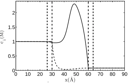
FIG. 4: Ion density profiles in the model, calculated for the following boundary conditions:
φ(−∞) =φ∞
L = 0;φ(∞) =φ∞R = -300 mV;n(−∞) =n∞L = 500 mM;n(∞) =n∞R = 40 mM; fixed
charge -0.227e in the middle of the channel normally distributed with standard deviationσ =0.1. Diffusion constants are DN a+ = DCl− = 2.09×10⁻¹⁰ m2/s. The vertical thin dashed-dot lines
indicate the position of the channel entrances. The vertical thick dashed lines show the boundaries for the calculations of access resistance.
the channel. In turn the PNP solution is determined by the concentrations and electrostatic potential at the channel mouth provided by the PBNP solution. This feature allows one to couple the PBNP solution in the bulk to the PNP solution in the channel in a self-consistent way, as described in the next sections.
IV. LINEAR APPROXIMATION
To appreciate that the boundary condition problem can be resolved uniquely, let us consider a linear approximation of the joint solution (9), (16), (26), (31), and (32). We note that, when both ion concentrations and fixed charge in the channel are relatively small, the last term in Eq. (9) can be neglected. In this approximation S1 = S0 = ref f2 ∇φP N P,
∇φP N P = φ1−φ0
[image:16.612.199.417.82.226.2]equations determines the boundary conditions as
φ1 =φ∞R −
ref fφx11−−φx00 −
PN
j=1zjβj
α/p
2nf
1 +p
2nfαref f
,
φ0 =φ∞L +
ref fφx11−−φx00 −
PN
j=1zjβj
α/√2
1 +√2αref f
,
βj =ref f2
Dj
2Db,j
Jjch=
zj(φ1−φ0)ref f2
x1 −x0
Dj
2Db,j
njL−njRezj(φ1−φ0)
ezj(φ1−φ0)−1 ,
(33)
where njL and njR are given by Eq. (26) at the surfaces of the boundary hemispheres
njL,R =n∞jL,R∓ βj
r.
This is the system of N + 2 equations with N + 2 unknowns (N unknown βj and two
unknown potentials at the channel entrances φ1 and φ0) and has a unique solution that
allows for the simultaneous solution of the access resistance problem and coupled Poisson and Nernst-Planck equations in the channel and in the bulk. Now we describe the algorithm for simultaneous solution of these equations in the more general nonlinear case.
V. JOINT SOLUTION
the form
φ(x) = (φ1−φ0) (x1 −x0)
(x−x0) +φ0 +
Z x1
x0
G(x, s)f(s)ds,
Jjch = njLe
zjφ0 −n
jRezjφ1
Rx1
x0 e
zjφ(s)ds ,
nj(x) =e−zjφ(x)
njLezjφ0 −Jjch
Z x
x0
ezjφ(s)ds
,
nj(r) = n∞j ∓
βj
r ,
φ(r) = (β+S0)e √
2α(aef f/d−r) 1 +√2αaef f/d
r − β
r +φ ∞
L,
φ(r) =−(βf +S1)e √2n
fα(aef f/d−r) 1 +p
2nfαaef f/d
r +
βf
r +φ ∞
R.
(34)
This leads us to the following algorithm for obtaining the self-consistent solution –
1. Initialization: Set the bulk values of the concentrations and electrostatic potential
on the left and right hand sides of the channel c∞
L, φ∞L, and c∞R, φ∞R respectively. Set
the potential to its initial value given by the linear function in Eq. (18).
2. PNP solution in the channel: (a) Calculate concentrations in the channel using
Eqs. (15) and (16); (b) Update the value of the potential using Eq. (9); (c) Repeat calculations from step 2(a) until convergence is reached; (d) Determine the currents inside the channel for each ion species, and calculate the electric field at the channel mouth;
3. PBNP solution in the bulk: (a) Update the value of the potential using Eq. (31);
(b) Calculate concentrations in the bulk using Eq. (24); (c) Use linear approximation in the boundary layer to determine the concentration and potential at the channel mouth;
4. Iteration Repeat steps 2 and 3 in turn until convergence is reached.
the fact that, in the zeroth approximation, the current through the channel and the electric field at the channel mouth have maximum possible values. At the next step this leads to the maximum possible reduction of the concentration and potential at the channel mouth. In turn, this reduces the current and electric field within the channel, which then leads to a smaller correction at the channel mouth; i.e. the scheme converges, leading to the solution shown in the Fig. 3. Note that in the two regions of thickness aef f (radius of the channel) on
the left and right hand sides of the channel, the gradient of the electric potential is assumed to be constant and equal to that in the channel. The corresponding density profile for two ionic species is presented in Fig. 4. As expected, the density profiles show a significant rise for Na+ and an abrupt decrease for the Cl− inside the channel. This suggests that the channel is most of the time occupied by a single Na+ ion but almost zero occupancy of Cl− ions, on average; we confirm this later when we estimate the channel occupation number as a function of membrane fixed charge and bulk concentration.
Another possible way of connecting the solution inside the channel to that in the bulk would be by matching the solutions asymptotically [33]. Although in a sense more interesting from the theoretical point of view, its use here would neither clarify our approach nor improve the quality of the fits to experimental results. It could, however, form the basis of a future project building on the ideas presented in the present paper.
A. Comparison with the experiments
The model is capable of reproducing experimental measurements if appropriate fitting parameters are used. These parameters include the distribution and magnitude of the chan-nel wall’s fixed charge, the ionic diffusion coefficient in the bulk and inside the chanchan-nel, and the filling factor described in Sec. (II D). The fixed negative charge on the membrane wall is taken equal to -0.227e. This corresponds to the number of particles inside the channel with a concentration of 250 mM. We stress that the projection of the distribution of fixed charge on the channel axis for the 1D approximation derived from the known 3D distribution of fixed charge has yet to be determined. The fixed charge is distributed along the 1D channel axis using a multimodal Gaussian distribution. With a suitable choice of these parameters, it is possible to fit experimental measurements for different concentrations.
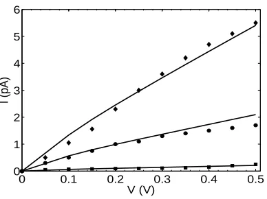
measure-ments by Oiki [43] in a 1M CsCl solution. The calculated current is given by the black thick line, while the experimental measurements are given by the circles. The calculated current is in good agreement with the experimental measurement. The robustness of this method is further tested by comparison with another set of experimental results presented by [44], as shown in Fig. 6. Again, good agreement is obtained between experiment and theory. Here, the (I −V) characteristics in the model are calculated for a channel with -0.227efixed charge distributed using a three mode Gaussian distribution. The fixed charge weights, positions and standard deviations are respectively: (-0.03e, -0.18e, -0.017e), (0.1, 0.5, 0.9), and (0.05, 0.10, 0.05). Ionic concentrations on both sides of the membrane are varied from 10 to 500 mM. Diffusion constants in the bulk areDb,N a+ = 1.33×10⁻⁹m2/s and
Db,Cl− = 2.03×10⁻⁹ m2/s. Diffusion constants in the channel are D
N a+ = 2.0×10⁻¹⁰ m2/s andDCl− = 0.95×10⁻¹⁰m2/s. The channel radius = 4 ˚A, length = 30 ˚A with a filling factor
of 0.1225 at 500 mM and 0.25 at 10 and 100 mM. Hollerbach, et al. [45, 46] used the spec-tral elements method to solve the 3D Poisson-Nernst-Planck equations for the Gramicidin channel. Portions of the bath were included into their simulations in order to have good boundary conditions. Their I−V characteristics at several symmetric concentrations were
−300 −200 −100 0 100 200 300 −15
−10 −5 0 5 10 15
I (pA)
[image:20.612.192.406.425.578.2]V (mV)
FIG. 5: Comparison of calculations with experiment. The full curve plots the current-voltage (I−V) characteristics (solid line) calculated for a channel with -0.227e fixed charge in its middle, normally distributed with a standard deviationσ =0.1. The ionic concentrations on both sides of the membrane is 1 M, and the diffusion constants are DCs+ = DCl− = 2.09×10⁻¹⁰ m2/s. The
0 0.1 0.2 0.3 0.4 0.5 0
1 2 3 4 5 6
V (V)
[image:21.612.209.403.77.222.2]I (pA)
FIG. 6: Comparison of calculated current-voltage (I−V) characteristics in the model (lines) with experimental data [44] for three different ionic concentrations, as follow: 10mM (filled squares), 100mM (filled circles) and 500mM (filled diamonds).
also compared to the same I −V curves measured experimentally by Andersen et al [44] and shown to be in good agreement.
Next we consider in more detail the dependence of the channel characteristics on other parameters.
VI. ANALYSIS OF THE CHANNEL PROPERTIES
In this section, we investigate the influences of the membrane fixed charge and the bulk concentrations on channel permeation.
A. Dependence on the channel fixed charge
The effect of the fixed charge variation on the channel is determined by calculation of the channel occupation number, the mean passage time, and the current for each ion species, as functions of the total fixed charge on the membrane wall (for given parameters of the fixed charge distribution). The occupation number Ci of the channel for each ion species is found
by integrating the corresponding concentration over the channel volume. For cylindrical geometry we have
Ci =fscπa2
Z L
0
˜
−0.20 −0.1 0 0.1 0.2 0.2
0.4 0.6 0.8
Occupation number
wall charge (units of e)
Na+
Cl−
N
Total
(a)
−0.210 −0.1 0 0.1 0.2
20 30 40 50
Mean passage time (nsec)
wall charge (units of e)
Na+
Cl−
(b)
−0.20 −0.1 0 0.1 0.2
1 2 3 4 5
I (pA)
wall charge (units of e)
Na+
Cl−
I
Total
[image:22.612.87.522.74.397.2](c)
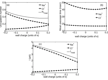
FIG. 7: Model calculations of (a) channel occupation number (b) ionic mean passage time and (c) ionic current, all as functions of the wall charge. The lines drawn through calculated points (filled circles for Cl− and filled squares for Na+) are guides to the eye, and the solid lines in (a) and (c) represent the total occupation number and the total current respectively. The applied voltage is 300 mV. Ionic concentrations in the left and right reservoirs are cL = 500 mM and cR= 40 mM,
respectively. Diffusion constants are DN a+ = DCl− = 2.09×10⁻¹⁰ m2/s. the channel radius =
4 ˚A, length = 30 ˚A with a filling factor of 0.28.
Note the filling factor in the expression for the occupation number. In general the filling factor has to be introduced individually for each ion species; however, for simplicity, we use here one average filling factor.
0.2 0.4 0.6 0.8 1 0
0.2 0.4 0.6 0.8 1 1.2 1.4
Occupation number
C (M)
(a)
0.2 0.4 0.6 0.8 1 10
20 30 40 50 60
Mean passage time (nsec)
C (M)
(b)
0.2 0.4 0.6 0.8 1 0
2 4 6 8 10
I (pA)
C (M)
[image:23.612.78.518.75.395.2](c)
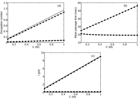
FIG. 8: Model calculations of (a) channel occupation number, (b) ionic mean passage time, and (c) ionic current, all as functions of bulk concentration. The lines drawn through calculated points (filled circles for Cl− and filled squares for Na+) are guides to the eye, and the solid lines in (a) and (c) represent the total occupation number and the total current respectively. The external potential difference was set to 300 mV with -0.227e fixed charge in the middle of the channel normally distributed with standard deviationσ=0.1. The ionic concentration in the right reservoir is cR = 40 mM; that in the left reservoir is allowed to change. Diffusion constants are
DN a+ =DCl−= 2.09×10⁻¹⁰m2/s. the channel radius = 4 ˚A, length = 30 ˚A with a filling factor
of 0.28
τM P S(i) =Cie/Ii, where Ii is the total current through the channel of the ion species i. Note
that this number corresponds to the total time one ion spends on average in the channel during the transition (in our example from left to right). The τM P S(i) differs from the usual mean first passage time by the factorCi.
of 500 mM and 40 mM, respectively, with an externally applied voltage of 300 mV. It can be seen from Fig. 7 that while the channel occupation number decreases for the cation as a function of the total wall charge, it increases for the anion. The conduction current decreases as a function of fixed charge for Na+ and increase for Cl− as the fixed charge increases and become positive. Note also that the total channel occupation numbers vary nonlinearly as functions of the fixed charge and are lower than 1 in the interval considered. The mean passage time shows a minimum for the anion, and decrease for the cation as the wall charge is increased. The motion of Cl− through the channel is slower than that of Na+. These dependences can be attributed to the charge affinity between the moving ions and the fixed charge distributed on the membrane wall. Estimation of the channel properties as a function of the channel fixed charge can be useful in gaining insight into the channel selectivity to specific ions as a result of the interactions between the ligand charge at the channel’s binding sites and the permeant ions. Furthermore, selectivity between alike ions within the PNP formalism can be obtained by introducing a separate filling factor for each ion species in order to take account of the ionic radius.
−0.26 −0.1 0 0.1 0.2
8 10 12 14 16
Conductance (pS)
wall charge (units of e) (a)
0.2 0.4 0.6 0.8 1 0
5 10 15 20 25 30 35
Conductance (pS)
C (M)
[image:24.612.91.520.402.562.2](b)
B. Dependence on the bulk concentrations
Fig. 8 plots the channel occupation number, ionic mean passage time, and ionic current in the channel, as functions of bulk concentration in the left-hand bath for an applied voltage of 300 mV. The concentration in the right-hand bath was kept constant at 40 mM. The channel occupation number increases linearly with the bulk concentration. The same variations are observed for the cation currents in Fig. 8 (c). As the bulk concentration increases, the Cl− current remain constant. This may be attributed to charge repulsion between the negatively charged protein (-0.227e) and the anion. We have ensured that the concentration changes investigated remain within the physiological range.
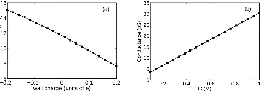
Fig. 9 calculates the channel conductance as a function of the wall charge and the bulk concentration. It is found that channel conductance decays as the wall charge increase, whereas it increases as the bulk concentration increases.
C. Diffusion-limited ion flow in the vicinities of the pore entrance
The AR as described by Hall [18],RHall = 4ρa, is used as the reference for our calculation.
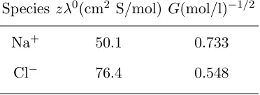
Here, ais the channel radius and ρis the resistivity of the solution. This corresponds to the resistance of the hemisphere close to the channel mouth which is of the same order as the one of the remaining infinite sphere in the case of an uncharged membrane. The conductivity of the electrolyte is expressed as the weighted sum of the equivalent conductivities λi and
given by ρ−1 = Pz
ic˜iλi [47]. The equivalent conductivities at 25 ◦C are approximated
by λi = λ
0
i
1+Gi√IM, that characterize concentration well and remain reasonably accurate at
concentrations near 1mol/l. The quantityIM = 12Piz2ic˜i is the ionic strength (molar basis).
The quantity λ0
i which is the equivalent conductivity of an ionic species at infinite dilution
and the empirical coefficients Gi are described by [48] and given in TABLE I:
Species zλ0(cm2 S/mol) G(mol/l)−1/2
Na+ 50.1 0.733
[image:25.612.213.399.617.685.2]Cl− 76.4 0.548
0.1 0.2 0.4 0.6 0.8 1 1
10 20 40 60 80 100
Access Resistance (G
Ω
)
[image:26.612.193.403.77.233.2]C (M)
FIG. 10: Access resistance (AR) calculated as a function of bulk concentration for a channel of radius 4 ˚A, length 30 ˚A, embedded in a negatively charged membrane, with charge -0.227e
distributed with a 1-mode Gaussian distribution of standard deviation σ =0.1, with the charges concentrated at the channel center, for a 300 mV external potential difference. The lines drawn through calculated points (filled circles for uncharged channel and filled squares for charged channel) are guides to the eye, and the solid line represent the Hall AR. The ionic concentration in the right reservoir is cR = 40 mM; that in the left reservoir is allowed to change. Diffusion constants and
filling factor are the same as in Fig. 8.
We have estimated the AR to the channel by considering the existence of voltage drops along the left and right mouth of the channel given respectively by ˜φL = ˜φ(˜x0)−φ˜∞L and
˜
φR = ˜φ∞R − φ˜(˜x1). The access resistances in the left and right hand mouths are given
respectively by RL =
˜
φL ˜
Ich and RR = ˜
φR ˜
Ich, where ˜I
ch is the total current through the channel.
The total AR to the channel is calculated as RT =|RL+RR |. We study diffusion-limited
presence of fixed charge on the membrane wall may result in the current saturation observed at high concentration.
VII. SUMMARY AND CONCLUSIONS
We have introduced a self-consistent analytic approach for calculation of the ion current through a channel and access resistance at the channel mouth as a function of the applied potential and bulk concentrations. In this approach the PNP solution in the channel is cou-pled to the PBNP solution in the bulk by matching the corresponding boundary conditions at the channel mouth in a self-consistent way and by introducing the “filling factor” as an additional fitting parameter that takes into account the radial distribution of current density in the channel. We note that this factor is introduced as a simple approximation of the free energy contribution due to the potential of the mean force in the channel. We note also that factors of this type are common in semiconductor theories (cf. the ideality factor in the diode equation [42]) that are used to model conduction in ion channels [33]. The method allows for calculation of the currents for an arbitrary number of monovalent ion species that have different diffusion constants in the channel and in the bulk. It is applied to fit experimental I−V characteristics of the Gramicidin A channel for various concentrations, yielding good quantitative agreement with the experimental results.
It is further shown that the changes in experimental I−V characteristics as a function of bulk concentrations can be successfully reproduced by the method. The corresponding changes in the filling factor can be attributed to the effect of saturation [49].
Given that the 1D PNP solution was earlier applied successfully to the analysis of exper-imental I −V characteristics in many ion channels [11–15], the scope of the present study also goes beyond the Gramicidin channel. In particular, with a subtle transformation of the channel structure, the work could be extended to other types of ion channel such as the L-type Ca2+ and Na+ channels. This implies adjustment of the concentrations and the fixed
charge on the channel wall. Because the filling factor allows for the ionic radius to be taken into account, it can be introduced for each ion species separately and the results obtained can also be used to gain further insight into the ion channel selectivity mechanisms that distinguish between alike ions.
of the solution of the PNP equations appeared in press [33]. In this approximation, which follows closely known asymptotic techniques of semiconductor physics [50], matching of the solution and boundary layers at the channel entrances is not required. However, the resultant analytical solution is discontinuous at the channel boundaries and for this reason is not well-suited to the estimation of access resistance discussed in the present paper. Besides, the approximation relies on charge neutrality, which was shown earlier to be a less accurate approximation to the numerical solution of the PNP in the bulk [21] than the linear approximation adopted here. The results [33] obtained for the constant charge density on the channel walls are not compared with experimental data. It will, however, be of interest to compare the two analytical approximations in the future.
The approach we have introduced can be further improved in a number of ways. First, the boundary conditions can be improved using e.g. the theoretical discussion in [22, 51]. More importantly the approach opens the possibility of an analytical treatment of the subtle details of the potential of the mean force revealed through molecular dynamics simulations (see e.g. [30]) but at the level of continuous PNP approximation. In particular, extending the idea of the filling factor, and including explicitly the PMF due to the wall vibrations and ion-wall interaction, will lead to a time-dependent Nernst-Planck equation with ˜ψP M F
j
specific for each ion species, thereby opening up the possibility of analytical insight into the selectivity of ion channels between alike ions. A model using Density Functional Theory (DFT) [52] to take care of finite size effects could also be used to patch the bulk solution.
ACKNOWLEDGMENTS
The work was supported by the Engineering and Physical Sciences Research Council (UK), the Russian Foundation for Fundamental Science, INTAS, and ESF.
[1] B. Hille, Ionic Channel Of Excitable Membranes, 3rd ed. (Sinauer Associates, Sunderland, MA, 2001).
[2] R. S. Eisenberg, Contemporary Physics39, 447 (1998).
[5] D. P. Chen, J. Lear, and R. S. Eisenberg, Biophys. J.72, 97 (1997).
[6] B. Corry, T. W. Allen, S. Kuyucak, and S.-H. Chung, Biophys. J. 80, 195 (2001). [7] B. Roux, Biophys. J. 71, 3177 (1996).
[8] V. Barcilon, SIAM Journal on Applied Mathematics 52, 1391 (1992), 0036-1399 Article type: Full Length Article / Full publication date: Oct., 1992 (199210). / Copyright 1992 Society for Industrial and Applied Mathematics.
[9] V. Barcilon, D. P. Chen, and R. S. Eisenberg, SIAM Journal on Applied Mathematics 52, 1405 (1992), 0036-1399 Article type: Full Length Article / Full publication date: Oct., 1992 (199210). / Copyright 1992 Society for Industrial and Applied Mathematics.
[10] S. Kuyucak, M. Hoyles, and S.-H. Chung, Biophys. J74, 22 (1998).
[11] D. P. Chen, V. Barcilon, and R. S. Eisenberg, Biophys. J.61, 1372 (1992).
[12] R. Elber, D. P. Chen, D. Rojewska, and R. Eisenberg, Biophysical Journal68, 906 (1995). [13] W. Nonner and B. Eisenberg, Biophys. J.75, 1287 (1998).
[14] D. P. Chenet al., Biophys. J.76, 1346 (1999). [15] R. S. Eisenberg, J. Membr. Biol 71, 1 (1999).
[16] S. M. Bezrukov and I. Vodyanoy, Biophys. J. 64, 16 (1993).
[17] J. Song, C. A. S. A. Minetti, M. S. Blake, and M. Colombini, Biophys. J.76, 804 (1999). [18] J. E. Hall, J. Gen. Physiol 66, 531 (1975).
[19] B. Hille,Ionic Channel Of Excitable Membranes(Sinauer Associates, Sunderland, MA, 1992). [20] M. S. P. Sansom and I. D. Kerr, Biophys. J69, 1334 (1995).
[21] A. Peskoff and D. M. Bers, Biophys. J.53, 863 (1988).
[22] V. Levadny, V. Aguilella, and M. Belaya, Biochimica and Biophysica Acta 1368, 338 (1998). [23] M. Aguilella-Arzo, V. M. Aguilella, and R. S. Eisenberg, Eur. Biophys. J 34, 314 (2005). [24] M. G. Kurnikova, R. D. Coalson, P. Graf, and A. Nitzan, Biophys. J. 76, 642 (1999). [25] G. Moy, B. Corry, S. Kuyucak, and S.-H. Chung, Biophys. J.78, 2349 (2000).
[26] A. Singer, Z. Schuss, D. Holcman, and R. S. Eisenberg, Journal of Statistical Physics 122, 437 (2006).
[27] D. Gillespie and R. S. Eisenberg, Phys. Rev. E63, 061902 (2001). [28] D. Gillespie and R. S. Eisenberg, Eur. Biophys. J34, 454 (2002).
[29] R. D. Coalson and M. G. Kurnikova, in Biological Membrane Ion Channels, Biological and
Krishnamurthy (Springer, New York, 2007), Chap. PoissonNernstPlanck Theory of Ion Per-meation Through Biological Channels, pp. 449–484.
[30] S. Y. Noskov, S. Berneche, and B. Roux, Nature 431, 830 (2004).
[31] D. Luchinsky et al., Journal of Physics: Conference Series, Electrostatics 2007 142, 012049 (2007).
[32] D. P. Chen and R. S. Eisenberg, Biophysical Journal65, 727 (1993).
[33] A. Singer, D. Gillespie, J. Norbury, and R. Eisenberg, Euro. Jnl of applied mathematics 19, 541 (2008).
[34] D. P. Chen and R. S. Eisenberg, Biophys. J.64, 1405 (1993). [35] S. McLaughlin, Anu. Rev. Biophys. Biophys. Chem18, 113 (1989). [36] D. P. Chen, J. Tang, and R. S. Eisenberg, Nanotech2, 64 (2002).
[37] R. S. Eisenberg, M. M. Klosek, and Z. Schuss, The Journal of Chemical Physics 102, 1767 (1995).
[38] C. Gardiner, Handbook of Stochastic methods for Physics and Chemistry, Number 13 in
Springer series in Synergetics (Springer, New York, 1996).
[39] H. K. Gummel, Electron Devices, IEEE Transactions on 11, 455 (1964), 0018-9383. [40] R. S. Eisenberg, J. Membrane Biol.150, 1 (1996).
[41] H. Monoi, Biophys. J.59, 786 (2005).
[42] S. Selberherr,Analysis and Simulation of Semiconductor Devices(Springer-Verlag, Wien, New York, 1984).
[43] S. Oiki, R. E. Koeppe II, and O. S. Andersen, Biophys. J. 66, 1823 (1994).
[44] O. S. Andersen, R. E. Koeppe, and B. Roux, IEEE Transactions on Nanoscience4, 10 (2005). [45] U. Hollerbach, D. P. Chen, D. Busath, and R. S. Eisenberg, Langmuir 16, 5509 (2000). [46] U. Hollerbach, D. P. Chen, and R. S. Eisenberg, Journal of Scientific Computing 16, 373
(2001).
[47] J. O. Bockris and A. K. N. Reddy,Modern Electrochemistry, Second Edition. Ionics (Plenum Press, New York and London, 1998).
[48] K. A. Snyder, X. Feng, B. D. Keen, and T. O. Mason, Cement and Concrete Research 3, 793 (2003).
[49] B. Corry, S. Kuyucak, and S.-H. Chung, Biophys. J.78, 2364 (2000).
(Springer-Verlag, Wien, New York, 1990).
[51] B. Eisenberg and W. Liu, SIAM J. MATH. ANAL38, 1932 (2007).