Water footprint of Indonesian provinces : the relation between water use and consumption in Indonesian provinces

(1)

(2)

Water Footprint of Indonesian

Provinces

The

relation

between

water

use

and

consumption

in

Indonesian

provinces

Bachelor Thesis

F. Bulsink April - July 2008

LabMath-Indonesia University of Twente

Bandung Enschede

(3)

Abstract

The demand for agricultural products will increase in Indonesia, but the agricultural sector is dealing with the problem of water scarcity. This study will analyze the water use in the agricultural sector and the consumption of this water by the population. In order to do so, the study will make use of the concept water footprint and virtual water content. The water footprint indicates how much water people directly and indirectly consume. The amount of water that a crop uses during its growth period is called virtual water content.

The program CROPWAT has been used for the calculation of the virtual water content in crops. The method for calculating the water footprint is developed by Hoekstra and Chapagain. Data for this study have been taken mainly from the years 2000 till 2004.

There is a big variety in the virtual water content of crops between provinces. Rice produced on Jawa has the lowest virtual water content of all rice in Indonesia. The green water component is relatively high for all crops, only for rice and soybeans the contribution of the irrigation water relatively high compared with the other crops.

The interprovincial virtual water flows are primarily caused by rice. The products cassava, coconut, bananas and coffee have the largest interprovincial water flows relatively to the water use for production. The biggest amount of virtual water from provinces or countries will go to Jawa. Sumatra has the largest contribution in the interprovincial water flows and the flows to other countries.

The average water footprint in Indonesia is 1092 m3/cap/yr, but there are large regional differences. The footprint varies between 841 and 1760 m3/cap/yr. The average water footprint consists for 84% of domestic internal water. The remaining 16% comes from other provinces or countries.

(4)

Preface

Four months ago I started with the preparations for my research and stay in Indonesia. After a short preparation period, I went to LabMath in Bandung to do research on the water footprint of Indonesia. In three month I managed to finish this research. It is a topic with a lot of interesting side steps, because of the limited time I only could finish my objective. Although improvements can be made, I am very content with the results.

I would like to thank a number of people for their support and guidance during this study.

First of all, I would like to thank my supervisors Martijn Booij, Sena Sopaheluwakan and Andonowati for their support, advice and guidance.

I would also like to thank everyone at LabMath-Indonesia, for their kindness and interest. I had a wonderful time at the institute and in Indonesia.

Next, I would also like to thank Gullit and Mees. With the three of us, we worked together on this subject. It was really inspiring, motivating and helpful. In the weekends we had a lot of time to explore the country together.

Finally, I want to say thank you to my family, friends and Hannah for their support during my period in Indonesia.

Rik Bulsink

(5)

Table

of

1 Introduction

1.1 Background

Agriculture is of great importance to Indonesia. The sector counts only for 11% to the GDP in 2002, but 44% of the labor force is working in the agricultural sector, making it the largest sector in terms of employment. Developments in this sector can lead to a reduction of poverty and the generation of broad-based economic growth (ADB, 2006). The sector has a strategic role concerning stability, economic growth and food security. To emphasize the important role of agriculture, the Ministry of Agriculture (2006) developed the following vision for the years 2005-2025: realizing a competitive, fair and sustainable industrial agricultural system to guarantee food security and community welfare. To develop the agricultural sector and achieve the abovementioned vision from the ministry, there are some challenges and problems to overcome. The agricultural sector is faced with increasing demand for agricultural products, caused by an increasing population and hence a higher consumption. Water resources for agricultural activities are also getting more scarcer, due to the impact of natural resources capacity degradation. Moreover, water use competition is also increasing due to increasing use of water for households and industries (Ministry of Agriculture, 2006).

To measure and analyze the water use by the agricultural sector and consumption of water by the population the water footprint has been developed.

The water footprint is a consumption-based indicator of water use and has been introduced by Hoekstra in 2002 (Chapagain & Hoekstra, 2004). This method indicates the water use of inhabitants from a country or province in relation to their consumption pattern. The traditional production-sector-based indicators show the water withdrawal in the domestic, agricultural and industrial sector. But this traditional method does not give information about the actual need of water by the people in a country in relation to their consumption pattern. So, the water footprint is a useful addition to the traditional production-sector-based indicators.

The concept of the water footprint is based on the principals of the ecological footprint, developed by Wackernagel and Rees (1996). The ecological footprint indicates the human demand on the Earth’s ecosystem and natural resources. It represents the area of productive land and aquatic ecosystems required to produce the resources used, and to assimilate the waste produced, by a certain population at a specified material standard of living, wherever on earth that land may be located. The ecological footprint shows the area needed to sustain people’s living, the water footprint indicates the annual water volume required to sustain a population (Chapagain & Hoekstra, 2004).

A nation’s water footprint exists of two parts, namely the internal and the external water footprint. The internal water footprint is defined as the use of domestic water resources to produce goods and services consumed by inhabitants of the country. The external water footprint is defined as the annual volume of water resources used in other countries to produce goods and services consumed by inhabitants of the country concerned (Hoekstra & Chapagain, 2007).

(8)

agricultural products, the industrial component corresponds with the water use for industrial products in the industrial sector and the domestic component is the water use in the domestic sector (Kampman, 2007). In this study the focus will be only the agricultural component.

The water footprint is closely linked to the virtual water concept. This concept has been introduced in the early 1990s by Allan (Allan, 1993). Virtual water represents the amount of water needed to raise a certain quantity of food (Allan, 1999). Virtual water is thus the amount of water that a crop needs during its growth and not the amount of water contained in the crop. The virtual water content of a product is measured at the place where the product is actually produced. Allan also suggests that trade of virtual water (coming along in the products) can release the pressure on the available water resources of a country. The water footprint is using the concept of virtual water in combination with the consumption rate of a population to determine the water consumption of this particular population. Virtual water content can be divided into a blue, green and gray component. The green component is the volume of water taken up by plants from the soil insofar it concerns soil water originating from infiltrated rainwater. The blue component refers to the water take up by plants from the soil insofar it concerns infiltrated irrigation water. The gray part covers the water required to dilute waste flows to such an extent that the quality of the water remains below agreed water quality standards (Chapagain et al, 2006b). The green and blue water footprints are based on Falkenmark (2003) and the gray component on Chapagain et al (2006b).

The water footprint has been calculated already for different countries by Hoekstra and Chapagain (2007). Indonesia is also included in this study. But for some countries, like India and China, further research have been done on a more detailed scale. Those studies give a better view of the water flows, consumption and use within a country than the study of Hoekstra and Chapagain. For Indonesia the detailed study has not been done yet, this study will be the first research about the water footprint of Indonesian provinces.

1.2 Objective

The objective of this study is to determine the water footprint of Indonesian provinces. The objective can be divided in the following sub questions:

1. What is the virtual water content of the crops cultivated in Indonesian provinces? 2. What are the virtual water flows between Indonesian provinces?

3. What are the water footprints of Indonesian provinces?

The study is focusing only on the production of agricultural products. The domestic and industrial water footprint contributes for only to about 10% to the global water footprint (Hoekstra & Chapagain, 2007).

This research is about the internal water footprint of Indonesian provinces and trade between Indonesian provinces. The external part of the water footprint has been studied by Mees Beeker. His work is about the flow of water into Indonesia and governmental policy in relation with virtual water. The report will start with an explanation of the used method in chapter 2. In chapter 3 the study area and the data will be given. The results of the calculation of the virtual water content can be found in chapter 4. In the next chapter the virtual water flows will be presented. In chapter 6 the water footprints of Indonesian provinces are presented. Chapter 7 contains the discussion and finally in chapter 8 the

(9)

2 Method

The method for determining the water footprint of Indonesia exists of several steps. First of all, the virtual water content of crops in the different provinces must be calculated. After the calculation of the virtual water content of primary crops, the calculation of the virtual water content of processed crops will be given. Subsequently, the calculation steps for the virtual water flows between provinces caused by trade will be shown. Finally, the water footprints of Indonesian provinces can be calculated. Throughout this chapter the following symbols will be used:

, 10

,

2.1 Virtual

water

content

Crops require a certain amount of water during their growth period. The actual amount of water that a crop uses is called virtual water. The virtual water content can be calculated in the following five steps: evapotranspiration, green crop water use, blue crop water use, gray crop water use and virtual water content.

2.1.1 Evapotranspiration

Evapotranspiration is a combination of two separate processes whereby water is lost on the one hand from the soil surface by evaporation and on the other hand from the crop by transpiration (Allen et al, 1998). The evapotranspiration , , / gives the amount of water evaporated by a crop under optimal conditions, there is an abundant of water in the soil. The , depends on location, crop and time. The formula for the evapotranspiration is as follows:

, , , , , (1).

Here, is the crop coefficient and is the reference evapotranspiration in a province /10 . For this calculation , is calculated for every time step of 10 days over the full growing period. The assumption is made that a month consists of 30 days.

The reference evapotranspiration is the evapotranspiration of a hypothetical grass. The only factors affecting are climatic parameters. Water is abundantly available at the surface and soil factors do not affect the . The depends on location and time. The will be calculated with the FAO Penman-Monteith method. The formula is as follows:

Δ

Δ 1

(2).

(10)

defined, cause this study is not focussing on this equation. Reference here can be made to the work of Gullit Widarta in which this equation is further researched and explained. This study will use this method, just like all the other studies related to the water footprint.

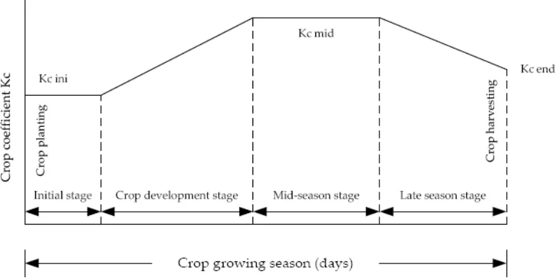
[image:10.595.97.500.190.393.2]

The reference evapotranspiration will be corrected by the crop coefficient . This coefficient depends on croptype, variety and development stage. The differences are mainly caused by the resistance to transpiration, crop height, crop roughness, reflection, ground cover and crop rooting characteristics. The crop development stage in relation with can be visualised as follows:

Figure 2.1: Development of Kc during the crop growing season (Chapagain & Hoekstra, 2004)

Here, the initial stage is the period from the planting date to approximately 10% ground cover, the crop development stage is the period from 10% ground cover to effective full cover, the mid-season stage is the time from effective full cover to the time the crop starts to mature and the late season is the time from the start of maturity to harvest.

2.1.2 Green crop water use

The green component is the volume of evaporated rainwater that is used for crop growth, the evapotranspiration. The green crop water use is the total amount of evapotranspiration of rainwater. The formula for the green crop water use , / is as follows:

, 10 , , ,

(3).

Here, , is the crop evapotranspiration under rain fed conditions / . The factor 10 is included to convert mm into m3/ha and the summation is done over the full lenght of the growth period

, in time steps of 10 days.

The crop evapotranspiration under rain fed conditions , , / is the evapotranspiration of rainwater by the crop and can be calculated as follows:

, , , , , , , (4).

(11)

the total rainfall minus runoff and deep percolation. Only the water retained in the root zone can be used by the plant and represents what is called the effective part of the rainwater. The effective rainfall is thus the fraction of the total amount of rainwater useful for meeting the water need of the crops (FAO, 1986).

2.1.3 Blue crop water use

The blue component is the use of groundwater and surface water for evapotranspiration during the production of a commodity. This component consists of evapotranspirated irrigation water. The blue component can be calculated as follows:

, 10 , , ,

(5).

Here, is the volume of irrigation water that is actually supplied to the crop field / and , is the actual crop evapotranspiration of irrigation water / . The factor 10 is included to convert mm into m3/ha and the summation is done over the full lenght of the growth period , in time steps of 10 days.

The actual crop evapotranspiration of irrigation water depends on the amount of irrigation water required by the crop and the fraction of land that is actually irrigated and foresees this requirement. This component can be calculated as follows:

, , , , , , (6).

Here, is the irrigation water requirement / and is the fraction of the total area of crop that is irrigated .

The fraction of total irrigated area can be derived from data. The calculation of the irrigation water requirement is as follows:

, , , , , , , , (7).

Only the irrigation water use on the field is taken into account, which means that the loss of irrigation water is excluded.

2.1.4 Dilution water requirement

The dilution water requirement is the amount of water that is required to dilute pollutants to such an extent that concentrations are reduced to agreed maximum acceptable levels during the production of the commodity. To stimulate the growth of a crop, fertilizers are applied to the crops. These fertilizers can be distinguished in nitrate, potassium and phosphorus. Only nitrate is taken into account in this study, because the mobility and the impact of the others are too low (Mom, 2007). The calculation of the dilution water requirement is as follows:

, , (8).

(12)

The factors determining the amount of nitrate that has leached to the groundwater are the amount of nitrate supplied to a field and the leaching factor. The calculation is as follows:

, , (9).

Here, is the total amount of nitrate supplied to the field / and is the leaching factor, which is the fraction of the total supplied amount of nitrate that eventually leaches to the groundwater

.

The dilution factor depends on the recommended level of nitrogen in the groundwater, the formula is as follows:

10 (10).

Here, is the dilution factor / and is the recommended level of nitrogen / . The factor 106 is added to the formula to convert l/mg into m3/ton.

2.1.5 Virtual water content

The virtual water content of a crop has three components, namely the green, blue and gray component. The calculation of the virtual water content is as follows:

, , , , (11).

Here, is the total virtual water content of a crop / , is the green virtual water content of a crop / , is the blue virtual water content of a crop / and

is the gray virtual water content of a crop / . The green component is calculated as follows:

, ,

,

(12).

Here, is the volume of the total rainfall that is actually used for evapotranspiration by the crop field / and is the yield of a crop / .

The blue component is calculated as follows:

, ,

,

(13).

Here, is the volume of irrigation water that is actually supplied to the crop field and used for evapotranspiration / .

The gray component is calculated as follows:

, ,

,

(14).

(13)

2.2 Virtual

water

content

of

processed

crops

The virtual water content of processed crops depends on the virtual water content of the primary crops. The virtual water content of the primary crop is distributed over the different products from that specific crop. The distribution model of virtual water over the products is based on the production fraction and value fraction. Distribution based only on the weight of product would be less meaningful (Chapagain and Hoekstra, 2004). For example, two processed products of the oil palm fruit are palm oil and the palm nut and kernel. The oil has a low weight fraction but a high value fraction, compared with the palm nut and kernels. The oil palm fruit is mainly cultivated for the oil. So if the distribution would only be based on the weight, the virtual water content of the processed products would be unrealistically distributed.

The production factor , of product is calculated as follows:

(15).

Here, is the weight of the processed product and is the total weight of the root (input) product .

The calculation of the value fraction , of product a is as follows:

∑

(16).

Here, is the market value of the processed crop $/ and is the production factor . The summation is to determine the aggregated market value of all products obtained from the root product. The virtual water content of the processed crop , / is calculated as follows:

, , (17).

Here, is the virtual water content of the root product in a province / .

2.3 Virtual

water

flows

Trade determines the external water footprint and thus virtual water flows. In this study two different sorts of trade are taken into account, international and interprovincial trade. The virtual water flow between provinces can be calculated with the flow of products between provinces and the virtual water content of these products. The international virtual water flow can be calculated with the flow of products between a province and a country and the virtual water content of these products. First, the method to determine the flows of products will be explained and after this the calculation of the virtual water flows. The trade model is based on the model used in the study of Ma et al (2006).

2.3.1 Trade

The calculation of the flow of products that are entering or leaving a province is based on the national food balance. The national food balance consists of supply and utilization. The domestic supply

, / of a crop is equal to the utilization , / .

(14)

, and , can be calculated as follows:

, , , , , , (19).

, , , , , , , (20).

Here, is the production quantity / , is the international import quantity / , is the stock increase / , is the stock decrease / , is the international export quantity / , is the feed quantity / , is the seed quantity / , is the manufacture quantity / , is the waste quantity / , is the other use quantity / and is the consumption quantity / .

The structure of the national food balance applies also for a province, the provincial supply , / is equal to utilization , / .

, , (21).

, and , can be calculated as follows:

, , , , , , , , (22).

, , , , , , , (23).

Here, is the interprovincial import quantity / and is the interprovincial export quantity / .

The difference between the national and provincial balance is that in the provincial balance also the interprovincial trade is taken into account. This is the mutual trade between provinces.

The production and consumption differs per province. For each province it is possible to calculate whether there is a surplus or a deficit of a certain crop. If the production is higher than the consumption there is a surplus. A deficit occurs if the consumption is higher than the production. The surplus of a crop in a province , / is calculated as follows:

, , , , , (24).

The crop seed use and crop waste are derived for the national balance and can be calculated as follows:

, ,

(25).

, ,

(26).

The crop waste and seed use are assumed as a fixed percentage of the total production.

(15)

is a positive surplus. With a surplus there will be no import and the export will be equal to the positive surplus. The export will be international as well as interprovincial. The surplus will be negative, if the consumption in a province is higher than the production. To fulfil the demand products will be imported. The import will be equal to the negative surplus and there will be no export. The import comes through international trade as well as interprovincial trade. This assumption about surplus, deficit and trade is confirmed by Mr. Arifin, senior economist at the Institute for development of economics and finance in Jakarta (personal communication, June 26, 2008).

The international export / and the interprovincial export / , in case of a positive surplus , / of crop c in province p, are calculated as follows:

, ,

(27).

, , _∑ ,

,

(28).

, , , , , ,

∑ ,

(29).

The summation will be done over the number of province that have a positive surplus of the crop (m) and / is calculated as follows:

, , , , (30).

These units apply to the country and can be derived from the national crop balance. The assumption is made that these units are relatively distributed over the provinces with a positive surplus.

In case of a deficit, negative surplus, , / the international import / and the interprovincial import / of crop c in province p are calculated as follows:

, , _∑ ,

,

(31).

, , , , ,

∑ ,

(32).

The summation will be done over all provinces (n) minus the provinces that have a positive surplus of crop (m).

The total interprovincial export is distributed over the total interprovincial import . The assumption is made that first it is distributed over the island groups, because of the relative short distance between provinces and the infrastructure on an island. Distribution will be done according to the relative seize of the surplus. The calculation of the flow of products from province 2 to province 1 is as follows:

, , , _∑ ,

, ,

(16)

The summation will be done over the provinces with a surplus in an island group (m). R is the sum of all the interprovincial import and export / . R can be calculated as follows:

, , , (34).

The summation will be done over all the provinces in an island group. The following distinction is made about R:

0 0

| | 0

After the distribution inside an island group, some provinces have still a surplus or deficit. The provinces with a surplus are distributed over the provinces with a deficit. The distribution will be based on the relative seize of the surplus and will be done over Indonesia. The formula is as follows:

, , , ,

∑ ,

(35).

Here, is the import from a province of crop c / , is the interprovincial export quantity of a province that is leftover after the first distribution / and is the deficit of provinces after the first distribution / . The summation will be done over all the provinces with the deficit after the first distribution (n).

2.3.2 Virtual water flow

The virtual water flow is the total amount of virtual water in the flow of traded products. The virtual water flow as result of crop trade between two provinces , / is calculated as follows:

, , , , , , , , (36).

Here, is the interprovincial export from province 1 to province 2 of a crop / , is the interprovincial import from province 2 to province 1 of a crop / and VWC is the virtual water content in the exporting province of crop c / .

The total virtual water flow between two provinces , , / is calculates as follows:

, , , ,

(37).

Here, the summation will be done over the total number of crops (n).

The net virtual water balance of a province is assessed in the form of the net virtual water import , / .

, ,

(38).

(17)

2.4 Water

footprints

The water footprint , / is the total volume of water needed to produce the goods that are consumed by the inhabitants of a province. The water footprint consists of an internal and an external part. The calculation is as follows:

(39).

Here, is the use of internal water resources to produce crops consumed by the inhabitants / and is the use of water resources of other province or other countries to produce crops consumed by the inhabitants of the province concerned / .

The internal water footprint , / footprint is calculated as follows:

(40).

Here, is the total agricultural water use in a province / and is the netto export of virtual water from a province / .

The external water footprint , / can be calculated as follows:

(41).

Here, is the net import of virtual water into a province / .

To make the results more comparble and determine the water consumption of the inhabitants of a province, the water footprint per capita , / / will be calculated as follows:

(42).

(18)

3 Study

area

and

Data

In the previous chapter the method has been explained, this chapter will focus on the data needed to carry out the calculations. Before the data will be presented, the study area will be explained.

3.1 Study

Area

[image:18.595.74.527.272.508.2]

Indonesia is an archipelago of 17,508 islands between the Indian Ocean and Pacific Ocean. Indonesia borders with Timor-Leste, Malaysia and Papua New Guinea. The total land surface covers 1 826 440 km2. Indonesia is located around the equator, the climate is therefore tropical. The total population of Indonesia is 237.512.355 (July 2008 est.). 59% of the total population is located on Jawa. The growth of the gross domestic product in 2007 was 6,3%. 43,4% of the labor force is employed in the agricultural sector, 18% in the industry and 38,7% is working in the services sector (CIA, 2008).

Figure 3.1: Map of Indonesia

(19)

[image:19.595.57.511.73.340.2]

Figure 3.2: Map of Indonesian provinces, special regions and district

In the past few years a couple of new provinces were created. In 2003 Papua Barat was split from Papua, in 2004 Sulawesi Barat was separated from Sulawesi Selatan and in 2004 the Riau Kepulauan were split off from Riau as a separate province. For the largest part of this research data from 2000 till 2004 are used, thus before the creation of these provinces. There was an overall lack of data about these new provinces, so the new provinces will not be taken into account for this study.

The provinces can be divided into 7 islands or island groups: Sumatra, Jawa, Lesser Sunda Islands, Kalimantan, Sulawesi, Maluku islands and Papua. Sumatra consists of Nanggroe Aceh D., Sumatera Utara, Sumatera Barat, Riau, Jambi, Sumatera Selatan, Bengkulu, Lampung, Bangka Belitung and Riau Kepulauan. Jawa consists of D.K.I. Jakarta, Jawa Barat, Jawa Tengah, D.I. Yogyakarta, Jawa Timur and Banten. Lesser Sunda Islands consists of Bali, Nusa Tenggara Barat and Nusa Tenggara Timur. Kalimantan consists of Kalimantan Barat, Kalimantan Tengah, Kalimantan Selatan and Kalimantan Timur. Sulawesi consists of Sulawesi Utara, Sulawesi Tengah, Sulawesi Selatan, Sulawesi Tenggara, Gorontalo and Sulawesi Barat. Maluku islands consists of Maluku and Maluku Utara. Finally, Papua consists of Papua Barat and Papua.

3.2 Crop

selection

(20)

[image:20.595.59.560.103.301.2]

Table 3.1: Crop categories and the production quantity, water use, production value and land use by category

Crop category Abbreviation Production Water use Production value Land use

M ton/yr M m3/ton % M US$/yr % M ha/yr %

Cereals CE 62,2 124885 49 8518 37,6 15,0 51,7

Oilcrops OC 65,5 67407 26 4484 19,8 6,9 23,7

Stimulants ST 1,3 16179 6 1023 4,5 1,9 6,7

Fruits FR 11,6 15693 6 3562 15,7 0,9 3,3

Roots and Tubers RT 20,8 9274 4 1469 6,5 1,6 5,5

Spices SP 0,4 8791 3 715 3,2 0,6 2,0

Nuts NU 0,2 5564 2 125 0,6 0,5 1,6

Sugarcrops SC 25,4 4577 2 475 2,1 0,4 1,5

Vegetables VE 6,7 3383 1 2230 9,9 0,9 2,9

Pulses PU 0,3 937 0 42 0,2 0,3 1,1

Total 194 256689 100 22644 100 29,0 100

For the study not all the crops will be taken into account, so the most important crops for this study are selected. The criterion for selection is that a crop should use more than 1% of the total water use. If an excluded crop has a production value above 5% or the land use is 2% or more, it will also be selected. The reason for the last two criteria is to make sure that important crops regarding land use and production value are not left out the study. The crops in table 3.2 are selected based on these criteria.

Table 3.2: Crop and the production quantity, water use, production value and land use per crop

Crop CC Production VWC Water use Production value Land use

1000

ton/yr

m3/ton M m3/yr % M US$/yr % 1000

ha/yr %

Rice, paddy CE 52015 2150 111832 43,57 7177 31,69 11643 40,21

Maize CE 10158 1285 13053 5,09 1341 5,92 3326 11,48

Cassava RT 17601 460 8096 3,15 1021 4,51 1276 4,41

Sugar cane SC 25173 164 4128 1,61 471 2,08 362 1,25

Cashew nuts, with

Shell NU 106 26788 2838 1,11 77 0,34 260 0,90

Soybeans OC 783 2030 1589 0,62 256 1,13 628 2,17

Groundnuts, with

Shell OC 1329 2231 2964 1,15 473 2,09 678 2,34

Coconuts OC 15796 2071 32714 12,74 921 4,07 2686 9,27

Oil palm fruit OC 47256 635 30008 11,69 2743 12,11 2673 9,23

Bananas FR 4297 1074 4615 1,80 1172 5,18 281 0,97

Guavas, mangoes,

mangosteens FR 1233 2264 2792 1,09 494 2,18 189 0,65

Fruit, nec FR 3546 1498 5312 2,07 1196 5,28 301 1,04

Coffee, green ST 623 17665 11012 4,29 445 1,96 1326 4,58

Cocoa beans ST 519 9959 5168 2,01 520 2,29 484 1,67

Cloves SP 94 66387 6235 2,43 298 1,31 346 1,19

Other crops 13851 14335 5,58 4039 17,84 2500 8,63

Total 194380 256689 100 22644 100 28957 100

[image:20.595.59.537.417.767.2]

(21)

The shaded crops are also excluded from the study because these are a leftover category. This category contains more than one crop or the crops belong to a category with a low water use. The selected crops belong to the five categories with highest water use.

The selected crops represent 86% of the total water use, 71% of the production value and 86% of the total agricultural land.

3.3 Data

Specific data about the selected crops and provinces are used for the calculation. In this paragraph the collection and use of these data will be explained

3.3.1 Population

The population by province is taken from BPS (2008a). The data apply to the year 2000. In Appendix I the population per province is given.

3.3.2 Climatic parameters

For the calculation of reference evapotranspiration and effective rainfall data about the climate are needed. With the program CROPWAT (FAO, 2008b) the reference evapotranspiration and the effective rainfall can be calculated. For the calculation of the reference evapotranspiration CROPWAT uses the FAO Penman-Monteith equation. The data for these calculations are taken from CLIMWAT (FAO, 2008c). In this database information is available from 33 weather stations across Indonesia. The data cover humidity, mean maximum and minimum temperature, wind speed, daily sunshine, rainfall and location (altitude, latitude and longitude) of the weather station. The data are given for each month in the year. The provinces and accompanying weather stations are listed in Appendix III. CLIMWAT does not provide enough weather stations, in some provinces there are no weather stations or the number of stations in a province is low. To get a reliable indication of the reference evapotranspiration and rainfall in all the provinces, supplementary data are used. These data are received from Badan Meteorologi dan Geofisika (BMG). BMG is the national weather institute of Indonesia. In Appendix III the supplementary weather stations are also listed.

For the weather stations Belwan, Jogjakarta, Kendari, Mengalla, Tahuna and Telukbentung, no data about the sunshine are available. The sunshine of nearby located weather stations are used as replacement. Furthermore, no weather stations are located in the province of Jambi. For Jambi the evapotranspiration is calculated as an average from the evapotranspiration in Riau and Sumatra Selatan, since those are two nearest-by provinces.

With these additional data from BMG, it is still no guarantee that the calculated reference evapotranspiration is the same as the actual reference evapotranspiration in a province. A cause for this difference could be the irregular distribution of those weather station across a province.

3.3.3 Crop parameters

The crop parameter (Kc) is used to correct the reference evapotranspiration, so the actual crop

evapotranspiration under optimal conditions is determined. The crop parameter contains the length of the crop development stages and the height of the Kc value. These parameters are based on Allen

(1998) and Chapagain and Hoekstra (2004). Because these sources contain general information for different climatic regions, additional information is used to determine the planting and harvesting date of the crops in Indonesia.

These parameters may differ per region in Indonesia, but for this study the parameters are taken as constant for every region within Indonesia. The assumption is made that a year has two seasons in Indonesia, a wet and a dry season. The wet season is from November till April and the dry season is from May till October. For annual crops the Kc value and the length of the growth period may differ per

(22)

3.3.4 Irrigated area fraction

Data about the fraction of the total area of a crop that is irrigated in a province is not available. That is why an assumption is made about this fraction. For every province data about land utilization, including the amount of wetland and dryland, is available (BPS, 2008b). Wetland is agricultural land that is irrigated, dryland is not irrigated and planted with seasonal crops. The estate crops, like oil palm, coconut, banana, coffee and cocoa, do not belong to these categories. Irrigation of these crops is not common (FAO, 1999) and information about this is not available.

To allocate the fraction of irrigated land over the crops in a province, the method as explained below is used. First of all, the irrigated land of rice is taken of the total wetland. Information about wetland rice is taken from the Ministry of Agriculture (2008). This information consists of the harvested area of wetland rice. Because it is possible to harvest rice at least two times a year, this area is divide by two. The surplus of land is distributed over the other crops based on relative area of these remaining crops, including the crops that are not taken into account for this study. For rice the irrigated area fraction is determined by dividing the area of wetland rice by the total area of rice, the sum of the area of wetland and dryland rice. The fraction of the total area of a crop that is irrigated is given in Appendix V.

For the provinces Maluku, Maluku Utara and Papua data about area of dryland and wetland are not available. This is the reason that the fraction of the total area of a crop that is irrigated is assumed to be 0. Only for rice the fraction of irrigation could be calculated, because data about wetland and dryland rice is available for these provinces.

3.3.5 Dilution water requirement

Data about fertilizer use are taken from Fertistat (FAO, 2008e) and FAO (2005). The data makes no distinction between provinces. Therefore it is assumed that the fertilizer use per hectare in every province is the same. Because of differences in yields between provinces, the gray virtual water content will not be de same for every province. The fertilizer use by crop is shown in Appendix VI. The leaching factor and recommended level of nitrate are taken from Chapagain et al (2006b). The leaching factor is assumed to be 10%. The recommended level of nitrogen is 10 mg/l, this is the standard recommended by EPA (2005) for nitrogen in drinking water.

3.3.6 Production quantity and harvested area

The production quantity and harvested area are taken from the Ministry of Agriculture (2008). In this database information about production quantity and harvested area from all the selected crops is available. The data makes distinctions between provinces. Data is taken from 2000 to 2004.

The figures are compared with the figures from FAOSTAT (FAO, 2008a) and BPS (2008c). Because the data from the Ministry of Agriculture for some products differs strongly with FAOSTAT en BPS, these numbers are corrected. The production quantity of coconut and oil palm and the harvested area of oil palm, banana and cocoa are corrected. The production quantity of these crops in the database from the Ministry of Agriculture represents processed crops and not the primary crops. The high harvested areas of these perennial crops were caused by the fact that these crops can be harvested several times a year.

The production quantity is shown in Appendix VII and the area is shown in Appendix VIII.

3.3.7 Weight and production fraction of processed crops

(23)

3.3.8 Food balance

The national food balance is taken from FAOSTAT (FAO, 2008a). The balance consists of domestic supply and domestic utilization. The domestic supply consists of production quantity, import quantity, stock variation and export quantity. The domestic utilization is feed quantity, seed quantity, food manufacture, waste quantity, other uses quantity and food quantity. For these quantities the average is taken from years 2000 till 2003.

The food balance is taken from FAOSTAT for the following products: rice (milled equivalent), maize, cassava, soybeans, groundnut (shelled equivalent), coconuts (incl. copra), palm kernels, soybean oil, groundnut oil, palm kernel oil, palm oil, coconut oil, bananas, coffee and cocoa beans.

In Appendix X the national food balance for Indonesia is shown.

No data about the consumption of a crop in a province is available. The assumption is made that each person consumes the same amount of a crop, independently of the location of living. The consumption, that is stated in the national food balance, is distributed over the provinces relative to the population.

3.3.9 Virtual water import

The import products from other countries will contain virtual water and will be a part of the water footprint. This international water flow coming into Indonesia is taken from Hoekstra and Mekonnen (2008). The virtual water import is an average of the years 2000 to 2003.

(24)

4 Virtual

water

content

With the method and data, as explained in the previous chapters, the virtual water content of the crops has been calculated. Firstly, the virtual water content of the primary crops will be given. Secondly, the virtual water content of the processed crops will be given and finally, there will be a comparison between these results and the result of previous studies.

4.1 Primary

crops

[image:24.595.83.523.258.449.2]

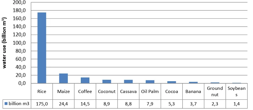
Before the virtual water content of the different crops will be presented, the water use of the crops will be given. Most water is being used for the rice production. This is caused by the high production quantity and the high demand of water for the production. In figure 4.1 the water use of the selected crops are shown.

Figure 4.1: Water use by product in billion m3

The virtual water content of the crops in a province are shown in Appendix XI. In each province the virtual water content is different, in some cases the differences are relative large. The differences are mainly caused by the evaportranspiration and yield. A high evapotranspiration contributes to a high virtual water content and a high yield will lead to a lower virtual water content.

The virtual water content in combination with the production will determine the average virtual water content of a crop in Indonesia. The virtual water content of cassava is the lowest of all crops, namely 497 m3/ton, and in coffee the highest, 22910 m3/ton. The other virtual water contents are listed in table 4.1.

Rice Maize Coffee Coconut Cassava Oil Palm Cocoa Banana Ground nut

Soybean s

billion m3 175,0 24,4 14,5 8,9 8,8 7,9 5,3 3,7 2,3 1,4

0,0 20,0 40,0 60,0 80,0 100,0 120,0 140,0 160,0 180,0 200,0

water

use

(billion

m

(25)

[image:25.595.72.402.94.274.2]

Table 4.1: Virtual water content of crops and the components

Crop Green Blue Gray Total

m3/ton

Rice 2460 668 212 3340

Maize 2315 68 13 2396

Cassava 471 7 19 497

Soybeans 1603 275 0 1878

Groundnut 2834 134 0 2968

Coconut 2838 0 16 2854

Oil Palm 797 0 51 848

Banana 849 0 0 849

Coffee 21907 0 1003 22910

Cocoa 8888 0 519 9406

The green component has the largest contribution to the virtual water content. The green component contributes for at least 85% of the total virtual water content, except for rice. For rice the green component is 74% of the total. The blue component is 20% for rice and 15% for soybean; for the other crops the contribution of the blue component to the virtual water content is marginal. Most crops are thus grown with rainwater. The crops rice, oil palm and cocoa have the largest gray component, because of the relative large amount of fertilizer application. This component counts for 6% of the total virtual water content for these crops.

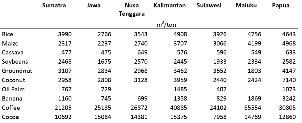
In table 4.2 the virtual water content of the crops over the island groups are shown. Rice from Jawa has the lowest virtual water content; maize and soybeans from Jawa also have a low virtual water content, compared to other island groups. Cassava from Jawa and Sumatra has the lowest virtual water content. Coffee has the lowest virtual water content when it is originated from Sumatra. The products which are produced in Sulawesi with a low virtual water content are coconut, oil palm and cocoa. Coconut has also a low virtual water content in Maluku. In Maluku groundnuts are also being produced with a low virtual water content. Bananas originating from Nusa Tenggara have the lowest virtual water content compared with the other island groups. The regional differences in virtual water content are caused by climate and yield.

Table 4.2: Virtual water content over the island group

Sumatra Jawa Nusa

Tenggara

Kalimantan Sulawesi Maluku Papua

m3/ton

Rice 3990 2766 3543 4908 3926 4756 4643

Maize 2317 2237 2740 3707 3066 4199 4968

Cassava 477 475 649 576 596 549 633

Soybeans 2468 1675 2570 2445 1933 2334 2582

Groundnut 3107 2834 2968 3462 3652 1803 4147

Coconut 2958 2808 3128 3959 2440 2424 7140

Oil Palm 767 729 1485 407 1073

Banana 1160 745 699 1358 829 1869 3242

Coffee 21205 25135 26872 40885 24102 85554 30805

[image:25.595.57.546.537.737.2]

(26)

[image:26.595.75.529.162.482.2]

Rice is an important and strategic crop in Indonesia. The virtual water content of rice is 3340 m3/ton, but there are big differences in the virtual water content in different provinces. Figure 4.2 illustrates these differences. 55% of the total rice production is produced on Jawa. Beside the provinces in Jawa, high producing areas are Sulawesi Selatan and Sumatra Utara. In these provinces the virtual water content is 3756 m3/ton and 3903 m3/ton. This is higher than the virtual water content of rice in Jawa, which has an average of 2766 m3/ton.

Figure 4.2: Virtual water content of rice in a province

4.2 Processed

crops

(27)

Table 4.3: Virtual water content of processed crops

VWC

m3/ton

Rice (Milled Equivalent) 5138

Soybean Cake 117

Soybean Oil 154

Groundnut shelled 4388

Groundnut Oil 6547

Copra 14271

Coconut Oil 5618

Palm Oil 8414

Palm kernels 18862

Palm kernel Oil 19821

4.3 Comparison

with

other

studies

[image:27.595.72.405.403.590.2]

Some other studies have already calculated the virtual water content of crops and also of crops in Indonesia. The comparison will be made with the results from Chapagain and Hoekstra (2004). This is the first study that calculated the virtual water content for each crop in a country. In table 4.4 the results of this study and the study from Chapagain and Hoekstra (2004) are listed.

Table 4.4: Virtual water content of this research and Chapagain and Hoekstra (2004)

This research Chapagain and Hoekstra (2004)

m3/ton

Rice 3340 2150

Maize 2396 1285

Cassava 497 460

Soybeans 1878 2030

Groundnut 2968 2231

Coconut 2854 2071

Oil Palm 848 635

Banana 849 1074

Coffee 22910 17665

Cocoa 9406 9959

(28)

5 Virtual

water

flows

The flows of products in combination with the virtual water content as calculated in the previous chapter will give the virtual water flows. Before presenting these flows, the food balances of the provinces will be given.

Provinces can have either a deficit or a surplus of a certain crop. A surplus will create an outgoing flow of a product or crop to other provinces or countries. A deficit on the other hand will create an ingoing flow of products into the province, these products can originate from either a province or a foreign country. In Appendix XII the surplus or deficit of a product in a province is listed, and also the amount of interprovincial and international import or export is listed. On the basis of this table a few remarks can be made relating to the production and flows. The table points out that there is a lot of interprovincial trade of rice, maize, cassava, coconut and bananas. The conclusion can be drawn that the production of some products is mainly regionally based. For example, Maluku Utara has a high production quantity of bananas and thus a large surplus; consequently there is an outflow of bananas from the Maluku towards the provinces with a deficit. Secondly, the products rice and soybeans rely on international import. The domestic production of these products is too low to meet the demand. Finally, the large exporting products are palm kernel oil, palm oil, coconut oil, coffee and cocoa.

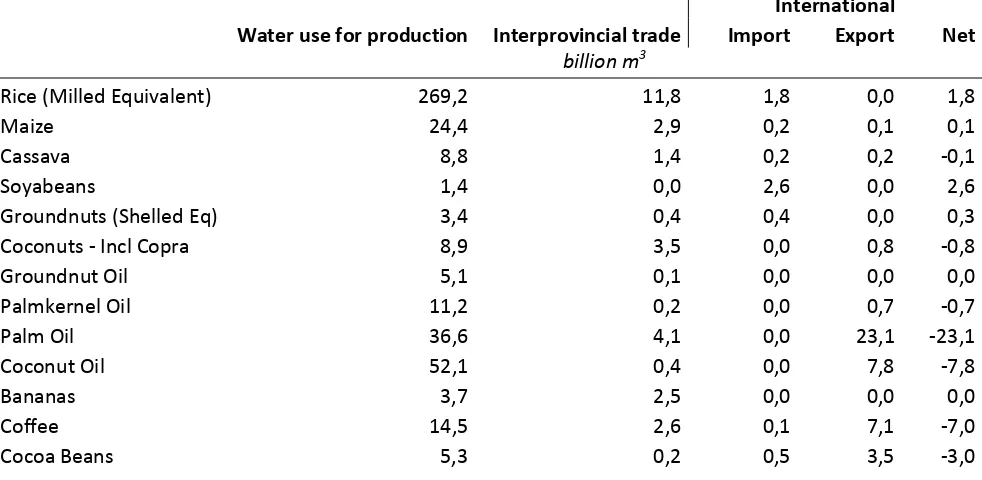
[image:28.595.60.551.449.689.2]

The flows of products also create flows of virtual water. In table 5.1 for each product the flow of virtual water is summarized. The difference between this table and Appendix XII is that this table represents the virtual water flow and the appendix shows the flow of a product quantity. The products with the relatively largest interprovincial flow of water are cassava, coconut, bananas and coffee. Bananas are by far the product with the largest interprovincial water flow relative to the water use for the production. Soybeans and groundnuts are the products with a high net import of virtual water. The products with a large amount of water that will leave the country are palm oil, coconut oil, coffee and cocoa beans.

Table 5.1: Water use and virtual water flows by crops

International

Water use for production Interprovincial trade Import Export Net

billion m3

Rice (Milled Equivalent) 269,2 11,8 1,8 0,0 1,8

Maize 24,4 2,9 0,2 0,1 0,1

Cassava 8,8 1,4 0,2 0,2 ‐0,1

Soyabeans 1,4 0,0 2,6 0,0 2,6

Groundnuts (Shelled Eq) 3,4 0,4 0,4 0,0 0,3

Coconuts ‐ Incl Copra 8,9 3,5 0,0 0,8 ‐0,8

Groundnut Oil 5,1 0,1 0,0 0,0 0,0

Palmkernel Oil 11,2 0,2 0,0 0,7 ‐0,7

Palm Oil 36,6 4,1 0,0 23,1 ‐23,1

Coconut Oil 52,1 0,4 0,0 7,8 ‐7,8

Bananas 3,7 2,5 0,0 0,0 0,0

Coffee 14,5 2,6 0,1 7,1 ‐7,0

Cocoa Beans 5,3 0,2 0,5 3,5 ‐3,0

(29)

total virtual water flow within Indonesia. These provinces have a large production and consequently a large surplus of one or more crops, so there is a big out flow of products to other provinces with a deficit.

According to Appendix XIII large interprovincial importing provinces are Jakarta, Jawa Barat, Jawa Tengah, Riau, Jawa Timur and Banten. These provinces represent 65% of the total interprovincial virtual water import. Because of the high consumption quantity and/or the low production of crops, these provinces have a high virtual water import.

The provinces Jawa Timur and Riau are both a large exporting and a large importing province. This is caused by the fact that the surplus of certain crops is high and the deficit of other crops is relatively large. For example, Riau imports a lot of rice and cassava and it has a large surplus in coconut and palm oil.

[image:29.595.28.548.312.483.2]

In table 5.2 the flows of virtual water between the island groups are represented. By far the most virtual water is imported in Jawa. The biggest interprovincial exporting island group is Sumatra.

Table 5.2: Flows of virtual water between provinces in million m3

Exporting

Sumatra Jawa Nusa

Tenggara

Kalimantan Sulawesi Maluku Papua Total

Importing

Sumatra 93 82 0 56 1 1219 1451

Jawa 7378 339 1472 3449 415 508 13560

Nusa Tenggara 340 1 95 105 0 0 540

Kalimantan 134 122 122 229 19 240 866

Sulawesi 61 122 20 15 16 298 532

Maluku 283 26 20 106 554 0 989

Papua 399 32 31 141 12 655 1272

Total 8596 396 613 1829 4404 1107 2266

The net virtual water flow is the export of virtual water into a province minus the import of virtual water originating of that certain province. In figure 5.1 the largest flows are visualized.

[image:29.595.74.534.568.740.2]

(30)

Besides the relatively small flows from and to Papua, the biggest flows are to Jawa. The largest flow of virtual water is from Sumatra to Jawa. The deficit of products on Jawa is causing this flow.

Noteworthy is the flow of virtual water from Papua to Sumatra. The virtual water flow is caused by the trade of bananas from Papua to Sumatra. It is uncertain if the flow is realistic. Because of the large distance between Papua and Sumatra, trade between the regions could be really low. It could be a limitation of working with this model.

[image:30.595.71.262.260.385.2]

The island group that exports the most water to other countries is Sumatra. The other island groups also contribute to the water export, but not as significant as Sumatra. The large flow of water out of Sumatra exists mainly of palm oil, coffee and coconut oil.

Table 5.3: International export of water by island group

International water

export (million m3)

Sumatra 29069

Jawa 933

Nusa Tenggara 1132

Kalimantan 5664

Sulawesi 5541

Maluku 541

Papua 653

(31)

6 Water

footprints

The water consumption of a person in Indonesia will be presented in this chapter. After that the distribution of the water footprints over Indonesia will be visualized and the contribution of the different crops to the water footprint is presented. Finally, there will be a comparison to other studies.

6.1 Water

footprint

of

Indonesian

provinces

[image:31.595.74.399.251.751.2]

In Appendix XIV the water footprints of the Indonesian provinces are shown. To make a better comparison between the provinces, the water footprint in table 6.1 is per capita.

Table 6.1: Water footprint per capita

Water footprint

Internal Interprovincial International Total

m3/cap/yr

Nanggroe Aceh D. 1196 72 4 1272

Sumatera Utara 1207 53 21 1282

Sumatera Barat 1083 69 24 1176

R i a u 658 457 80 1196

J a m b i 1279 131 35 1444

Sumatera Selatan 1179 106 31 1316

Bengkulu 1592 93 20 1706

Lampung 1159 5 19 1183

Bangka Belitung 352 620 109 1081

D.K.I. Jakarta 5 720 116 841

Jawa Barat 685 152 29 866

Jawa Tengah 1015 75 17 1106

D.I. Yogyakarta 898 152 19 1069

Jawa Timur 847 49 3 899

Banten 788 233 51 1072

B a l i 892 54 15 961

Nusa Tenggara Barat 1145 90 6 1240

Nusa Tenggara Timur 859 301 59 1220

Kalimantan Barat 1626 97 30 1753

Kalimantan Tengah 1538 181 41 1760

Kalimantan Selatan 1261 86 24 1371

Kalimantan Timur 1080 279 52 1410

Sulawesi Utara 992 192 38 1222

Sulawesi Tengah 1332 65 22 1419

Sulawesi Selatan 1199 30 13 1242

Sulawesi Tenggara 1058 213 43 1314

Gorontalo 908 250 39 1197

Maluku 367 554 90 1011

Maluku Utara 795 428 77 1300

Papua Barat 381 578 89 1048

(32)

The average water footprint in Indonesia is 1092 m3/cap/yr. People in Kalimantan Tengah have the largest water footprint, 1760 m3/cap/yr, and a person in Jakarta has the smallest water footprint, 841 m3/cap/yr. A person in Jakarta also relies the most on external sources. The imported products come most of all from provinces with a large surplus. The virtual water content in those products is relatively low, because the crops are efficiently produced with a high yield. This is causing the relatively low water footprint. Lampung has the highest use of internal water resources (98%). Lampung can fulfill its own needs for almost every crop, only for groundnuts and soybeans it has a small deficit. The provinces have an average internal water use of 84%, for the other 16% they rely on other provinces or countries.

[image:32.595.74.529.320.636.2]

In figure 6.1 the water footprints and their distribution over Indonesia are visualized. The water footprints on Jawa are relatively low, Kalimantan has a relatively high water footprint. The factors that determine the water footprint in general are: volume of consumption, consumption patterns, climate and agricultural practice (Hoekstra and Chapagain, 2008). Because in this study the volume of consumption per capita and consumption patterns are the same for each province, the differences in water footprints are caused by climate and agricultural practice. Agricultural practice has influence on the yield and thus virtual water content. In Jawa the yields are high and the evapotranspiration rate is lower compared with other regions, this is causing the low water footprint in Jawa.

Figure 6.1: Water footprints and distribution over Indonesia

6.2 Contribution

of

crops

to

the

water

footprint

(33)

[image:33.595.174.432.85.267.2]

Figure 6.2: Contribution of crops to the water footprint

The figure points out that rice contributes most to the water footprint. This is caused by the high virtual water content of rice, but also the high consumption rate of rice in Indonesia. Coconut and coconut oil also have a notably large contribution.

[image:33.595.82.519.444.686.2]

The crops contribute differently to the water footprint in different island groups. This is presented in figure 6.3. The contribution of rice is the highest in Kalimantan and Sumatra, namely 72%, and in the Maluku it is only 62%. Other remarks can be made that the coffee contribution in Papua is 12% and in the Maluku coconuts contribute for 15% to the water footprint.

Figure 6.3: Water footprints and contribution of crops for island groups Rice (69%)

Maize (6%)

Cassava (2%)

Soybeans (2%)

Groundnuts (2%)

Coconuts (10%)

Oil Palm (3%)

Bananas (2%)

Coffee (3%)

Cocoa Beans (1%)

0 200 400 600 800 1000 1200 1400 1600 1800

Water

footprint

(m

3/cap/yr)

Cocoa Beans

Coffee

Bananas

Oil Palm

Coconuts

Groundnuts

Soybeans

Cassava

Maize

(34)

6.3 Comparison

with

other

studies

[image:34.595.69.454.179.259.2]

Previous studies also calculated the water footprint. These studies calculated the water footprint for Indonesia as a whole and not for each province separately. The results of this study will be compared with results from Chapagain and Hoekstra (2004). For the comparison the average Indonesian water footprint will be used. In table 6.2 the water footprint of both studies are shown.

Table 6.2: Water footprint of this research and Chapagain and Hoekstra (2004)

This research Chapagain and Hoekstra

m3/cap/yr

Water footprint 1092 1317

Internal part of Agricultural goods 1063 1153

External part of Agricultural goods 28 127

(35)

7 Discussion

In this chapter the limitation of this study will be discussed. Based on this discussion, some recommendations for improvements and for further research will be made. These recommendations will be discussed in section 8.2

A sensitive part of this study is the climatic data. In the database from CLIMWAT (FAO, 2008c) not enough weather stations are available to get the country completely covered. Additional data from BMG is used to get a complete coverage. The average evapotranspiration of CLIMWAT is lower than the evapotranspiration from the BMG data. This can be caused by the distribution of the weather stations over the country and the corresponding climatic differences, but there is a possibility that the sources use different assumptions for collecting and processing the data. This could affect the entire calculation. Besides this it is also uncertain that the calculated evapotranspiration represented the actual evapotranspiration in a province.

In this study the water footprint is determined by provinces, this is a relatively accurate level. But sometimes data was not available on this level, for example the consumption rate and fertilizer use in provinces. In the study the assumption is made that these parameters are equally distributed over the provinces, of course it is not realistic to assume that these rates are equal in every province. For example, in Papua the main food is not rice but sweet potatoes, so the consumption of rice per capita would be lower than the average consumption. It is also assumed that the crop calendar and crop coefficient are equal in Indonesia as a whole. To improve the calculation accurate data and parameters by province are necessary.

The virtual water content of crops varies between provinces. For some crops the differences between provinces are not large. But for some other crops the difference is conspicuous large. For instance, rice has a virtual water content of 2766 m3/ton in Jawa and in Kalimantan the virtual water content is 4908 m3/ton. The yield and climate differences between those two regions have an influence. Still it is a large difference for the main crop in Indonesia.

The differences between the water footprints are also large. On Jawa the water footprint is low compared with the other regions. The difference between the province with the lowest water footprint, Jakarta, and the highest, Kalimantan Tengah, is more than double. Jakarta is a developed city and has probably an high consumption rate per capita. But in this study the consumption rate is equal over Indonesia and only the yield and climate data have influence on the water footprint. That is a reason why Jakarta has the lowest water footprint. However the real water footprint of a person in Jakarta will be higher than in this report.

For the calculation some crops are selected, so not all crops are taken into account in this study. To improve the study other crops could also be taken into account. The import of virtual water is especially lower because of this selection, since evident imported crops as cloves, wheat and sugar cane are not taken into account. Reference here can be made to the work of Mees Beeker (2008) in which the external water footprint will be calculated more accurately.

The trade distribution within Indonesia is unknown. For this study the model from Ma et al (2006) is adapted and used. It is hard to describe trade in a model when no data about interprovincial trade is available, because in a free market trade depends on many factors. When using different models, it would be possible to see the change in flows and the difference in results.

(36)

8 Conclusions

and

recommendations

8.1 Conclusions

The average water footprint of Indonesia is 1092 m3/cap/yr, but there are large regional differences. The footprint in Jakarta is the lowest, namely 841 m3/cap/yr, and the highest water footprint can be found in Kalimantan Tengah, 1760 m3/cap/yr. The provinces have an average internal water use of 84%, for the other 16% they rely on other provinces or countries. The factors that determine the water footprint are: volume of consumption, consumption patterns, climate and agricultural practice (Hoekstra and Chapagain, 2008). Because the consumption volume and pattern are the same for every person in each province, the differences in water footprint are caused by climate and agricultural practice. The provinces are for a small part depending on external water resources. Only Jakarta is highly depending on external water resources. The provinces depend only for 16% on water resources of other provinces or countries. The biggest contribution to the water footprint is rice. This is caused by the high consumption rate and the high virtual water content of rice.

The virtual water content varies within the country, there are large differences between provinces. For instance, of all big rice producing provinces, the provinces on Jawa have the lowest virtual water content. The virtual water content of rice produced on Jawa is almost half the amount of virtual water of the rice produced on Sulawesi Selatan or Sumatra Utara .The green water component has the largest contribution. The blue water use is for most products less than 15% of the virtual water content, only for rice and soybeans the blue water contribution is higher. Blue water use is affecting the environment more than the green water use, because this component is originating from groundwater or surface water. However, to ensure high yields and food security, irrigation water is required. The gray component is relative low, it contribute to at most 6% of the virtual water content. If the use of fertilizers will increase, this component will become a more important factor in the total virtual water content.

The interprovincial water flows are primarily caused by the trade of rice. The products cassava, coconut, bananas and coffee have the largest interprovincial flow relative to the water use for production. Sulawesi Selatan has the largest contribution to the interprovincial trade. The flow out of this province exists primarily of virtual water from rice. Large importing provinces are Jakarta, Jawa Barat, Jawa Tengah, Riau, Jawa Timur and Banten. The largest flow of net virtual water is from Sumatra to Jawa. Sumatra also exports the most virtual water to other countries. The large flow of water out of Sumatra exists mainly of the products palm oil, coffee and coconut oil.

Provinces depend highly on internal water resources. On average 84% of the water footprint consists of internal water, the trade and flow of water between provinces are low. There is a large variance between the virtual water content of products in provinces. In some provinces the production will take less water than in other provinces, thus the production is more efficient in those provinces. When the pressure on the resources will increase and water will become scarcer, trade of virtual water can save water, drop the pressure on the water resources and assure a high degree of food self-sufficiency within Indonesia. But to achieve this the agricultural sector needs to be reformed on the basis of water efficiently production. This will cause more trade between provinces and could lead to a lower water footprint.

8.2 Recommendations

(37)

Mom (2008) already included satellite data in his study about the virtual water content of rice. This method and data could ensure a more reliable and accurate result.

In the study consumption rate and pattern are equal over whole Indonesia, because no data was available per province. In general consumption rate and consumption pattern are related to income and wealth. If a model was available that uses those parameters, there would be variation in consumption rate between provinces. The water footprint would depend also on consumption rate and the result would be more realistic.

Water footprint of Indonesian provinces : the relation between water use and consumption in Indonesian provinces