A New Anytime Dynamic Navigation Algorithm

(1)

A New Anytime Dynamic Navigation Algorithm

Weiya Yue, John Franco, Weiwei Cao

∗

, Qiang Han

Abstract—Dynamic navigation algorithm has been an impor-tant component in planning. Navigation algorithm is required to find out an optimal solution to its goal. However, under some environments where time is more critical than optimality, a sub-optimal solution is acceptable. Therefore for practical applications it is useful to find a high sub-optimal solution in limited time. The dynamic algorithm Anytime D*(AD*) is currently the best anytime algorithm which aims to return a high sub-optimal solution with short corresponding time and control of sub-optimality. In this paper, a new algorithm named Improved Anytime D*(IAD*) is introduced. Experiment comparison is made to show IAD* better outperforms Anytime D* in various random benchmarks.

Index Terms—Planning, Dynamic Navigation Algorithm, Anytime, Incremental

I. INTRODUCTION

W

ITH development of techniques, it is highly possible to develop autonomous vehicles, intelligent agents, etc. Because of this, navigation algorithm has been more and more important. In navigation algorithm, an agent is required to find out one optimal solution to its goal under changing environment. Many algorithms have been developed to solve this problem and gained big success [1], [2], [3], [4], [5], [6], [7]. But under some environments, where there is no sufficient resources for the agent to find out an optimal solution, a sub-optimal solution is acceptable. In this paper, we will focus on the environment where time is more critical than optimality.

Time-limited search algorithms, called anytime planning algorithms, have been developed to fit in time critical envi-ronment. The basic idea is to find one solution as soon as possible, then to progressively replace a stored path with a better path when one is discovered during search until the time available for search expires [8], [9], [10]. Then the stored, probably sub-optimal path is the one that is used. In [8], [11], [12], it has been demonstrated that a so-called weighted A* algorithm variant which uses “inflated” heuristics (described below) can expand fewer vertices than the normal A* algorithm.

In A*, the vertices in OP EN are sorted by their values f = g+h. By assuming h is admissive, in A* algorithm if we use f = g+ϵ·h, then the returned path can be guaranteed to beϵsub-optimality, i.e.g(vg)≤ϵ·g∗(vg)[13]. This strategy is called inflated heuristics, and the benefit is the control of ϵ sub-optimality. The A* algorithm us-ing inflated heuristics is named weighted A* algorithm. In [8], one general method, named Anytime Weighted A*, to transform heuristic search algorithms to anytime algorithms

Manuscript received August 18, 2012.

W. Yue and J. Franco and Q. Han are with the Depart-ment of Computer Science, University of Cincinnati, Cincinnati, OH, 45220 USA e-mail: [email protected], [email protected], [email protected].

W. Cao is with Institute of Information Engneering, Chinese Academy of Science, Beijing, China, 100093 e-mail: [email protected].

is proposed. Anytime Weighted A* is a anytime planning algorithm which returns one sub-optimal solution as soon as possible then whenever allowed continues to improve current solution until one optimal solution returned.

Anytime Weighted A* does initialization on most variants as A* algorithm, and as Weighted A*, the heuristic function hused is admissive. Different from normal A* algorithm, in Anytime Weighted A* pis used to record current returned path which may be improved later; ERROR is used to estimate how far away current solution is from optimal path; ϵ is the parameter used to inflate h; in one vertex v ∈ OP EN, the stored values are ⟨g(v), f′(v)⟩ instead of ⟨g(v), f(v)⟩, in whichf′(v) =g(v)+ϵ·h(v). I.e., in Anytime Weighted A* in priority queue OP EN, the vertices are sorted byf′value instead offvalue in normal A* algorithm. Although Anytime Weighted A* uses inflated heuristic value f′ to sort vertices, normalf values are also recorded, which is used to prune searching space [9].

Under the changing environment, to search a path between a fixed pair of vertices within limited time, incremental any-time algorithm Anyany-time Repairing A*(ARA*) algorithm [14] was developed to mitigate this problem. ARA* runs weighted A* algorithm many times. Every time changes observed, ARA* needs to run weighted A* to find the new sub-optimal path. Most important to the performance of ARA* is that it reuses previously calculated information to avoid duplicating computation. This is done in accordance with ideas taken from [15], [16]. By observing that in weighted A* when h is admissive, if every vertex is allowed to be expanded only once, the returned path is still ϵ sub-optimal, every time ARA* needs to recalculate, ARA* will only update a vertex at most one time. ARA* starts with a large value for the so-calledinflated parameterϵand then reducingϵon each succeeding round until either ϵ = 1 or available time expires. ARA* performs similarly as Anytime Weighted A* algorithm and give the ability to control the sub-optimality ϵ.

D* Lite algorithm can be treated a dynamic version of lifelong A* algorithm [15], [16]. As D* algorithm [3], [4], D* lite searches backward fromvg tovs. This is likely the critical point to the success of D* and its descendants because theg value of every node is exactly the path cost from that node to the goalvg and can be usedafter the agent moves to its next position. The functionrhsis defined by

rhs(v) = {

minv′_∈succ(v)g(v′) +c(⟨v, v′⟩) v̸=vg

0 otherwise,

(2)

by following the maximum-g-decrease-value vertices one by one from target vg. If some changes that have been made since the last round cause a vertexv to become inconsistent then D* Lite will update g(v) to makev locally consistent by setting g(v) = rhs(v). Because D* Lite algorithm will only propagate inconsistent vertices to update partial vertices’ (g, rhs) values instead of updating all vertices’ (g, rhs)values, D* Lite can perform much better than other navigation algorithms.

Anytime D* [17] intends for dynamic navigation ap-plications where optimality is not as critical as response time. It may be thought of as a descendant of both the Anytime Repairing A*(ARA*) and D* Lite algorithms. It may re-calculate a best path more than once in a round with decreasing ϵ-suboptimality until ϵ= 1 or time has run out. Thus, Anytime D* will try to give a relatively good, available path quickly and, if time allows, will try to improve the path incrementally as is the case for Anytime A*.

In [5], [6], D* Lite algorithm has been improved by avoid-ing unnecessary calculations further, in which if the original optimal path is still available and can not be improved by changes observed, that path will be chose without computing. In [7], the ID* Lite algorithm uses a threshold number which is estimated to control the propagation of inconsistent vertices. Every time only changes may contribute a path whose weight is less or equal with the threshold number are propagated. The threshold number is increased until an optimal path found or all inconsistent vertices have been updated.

In this paper, we will combine the techniques used in ID* Lite to improve Anytime D* algorithm and get an algorithm names Improved Anytime D* algorithm, and IAD* for abbreviation. In Section II, pseudo code of IAD* is listed and described. Then in Section III, IAD* and AD* are compared in various random benchmarks. At last, we concludes and discuss the next step of work.

II. IMPROVEDANYTIMED* ALGORITHM

In this section at first we explain how IAD* algorithm works and then give its pseudo code. As Anytime D* algorithm, when changes observed, IAD* will try to update inconsistent vertices to get a new sub-optimal date. Every time, after recalculating, it is required to return a sub-optimal path whose weight is no bigger than ϵ′ ·g∗ in which ϵ′ is a preset parameter to control sub-optimality and g∗ is the weight of current optimal path.

Every time, when recalculating needed, the sub-optimality parameterϵis reset to beϵ′ which is relatively big. By doing this, we expect to return a path as soon as possible [8], [12], [11]. In [18], it is recommended that in weighted A*ϵ can be set to be bigger thanϵ′ and experiments show that the first path can be returned faster. This technique can be combined with any weighted A* algorithm easily. In order to speed up returning the first path, Anytime D* allow one vertex to be expanded at most one time which will be explained later. But it has been shown that in some benchmarks this may delay propagation of some critical vertices and slow down the algorithm [8]. In Section III, we will run experiments to compare these results.

After the first path returned, as any other anytime algo-rithm, IAD* will try to improve current path until time runs

out or an optimal path has been found. In Anytime D*, in order to do so, ϵ is decreased to look for a new path until ϵ= 1which means the returned path is optimal. When ϵis decreased, in Anytime D* all inconsistent are inserted into priority queue to be updated. As in ID* Lite [7], IAD* will not do any recalculating at all. Given aϵ, at first, IAD* will try to find one consistentϵ′ sub-optimal path which is not affected by changes observed, and if such a path exists, it is returned immediately as the first path found. If no such a path found, IAD* will only choose part of overconsistent vertices whose propagation may lead to aϵsub-optimal path. The pseudo code of IAD* is listed in Figure 1. Function

Initialize() defines and initializesϵ, and the priority queues OPEN, CLOSED, and INCONS, and initialize values forg, rhs and type values of vertices. The initial value of ϵ0 is relatively large in order to make sure some path is returned quickly. And vertex vg and itskey is inserted into priority queue OPEN.

In Function key(s), under-consistent vertices have their key-values updated as g(s) + h(s) which is smaller than

key(vs). This processing can guarantee such kind of increas-ing changes can be propagated. Function UpdateVertex(s) updates one vertex in the same way as Anytime D* by using INCONS to store some of the inconsistent vertices and making sure that one vertex is expanded at most once in one execution of ComputeOrImprovePath(). After doing this, there is still returned solution generated satisfies ϵ -suboptimality [17].

Functions ComputeorImprovePath(), MiniCompute() andGetBackVertex(v)are the same as in ID* Lite. Function

GetAlternativePath(vc) returns TRUE if and only if there is a path from vc to vg and, if it returns TRUE, it has changed type values on vertices so that a least cost path from vc to vg can be traversed by visiting neighboring vertices of lowest positive type untilvg is reached. Different from ID* Lite, at line 05, instead of choosing a child of r, one successory of rwithrhs(y) +c(r, y) ≤rhs(r)is chose. The reason is that here we only need a suboptimal path.

Different from ID* Lite, here the returned path may be not optimal, but is guaranteed to be ϵ′ suboptimal. It worths to notice that if a path returned, and on which there are overconsistent vertices, then the path returned is better than ϵ′ suboptimal. If no path can be returned by function GetAlternativePath(vc), every vertex c ∈ C is updated by function UpdateVertex. Observe that c is underconsistent and that this is the only place in the code where underconsistent vertices are placed in OPEN as in ID* Lite [7]. This is because only increased changes will cause underconsistent vertices, and increased changes are only inserted here. Decreased changes have been inserted beforeGetAlternativePath(vc) was called.

ProcessChanges acts similarly as ID* Lite. But differ-ently, at line 07 and 17, to test whether a overconsistent vertex should be put in OPEN to propagate, ϵ∗h(vc, u) + rhs(u) < t is used instead of h(vc, u) +rhs(u) < t. FunctionsMain() andMoveAgent() are the same as Anytime D*.

We end this Section with the Theorem of correctness of IAD*.

(3)

Procedure Initialize()

01. OPEN = CLOSED = INCONS = catch=∅;

02. for allv∈V,rhs(v) =g(v) =∞;type(v) =−1; 03. rhs(vg) =g(vg) =type(vg) = 0;ϵ=ϵ0

04. OPEN.insert([vg, [h(vg),0]]);

Procedure key(s): 01. if (g(s)> rhs(s))

02. return[rhs(s) +ϵ·h(s), rhs(s)]; 03. else

04. return[g(s) +h(s), g(s)];

Procedure UpdateVertex(s): 01. ifshas not been visited 02. g(s) =∞;

03. if (s̸=vg)rhs(s) =mins′∈succ(s)(c(⟨s, s′⟩) +g(s′));

04. if (s∈OPEN) OPEN.remove(s); 05. if (g(s)̸=rhs(s))

06. if (s∈CLOSED)

07. OPEN.insert([s,key(s)]);type(v) = 0; 08. else

09. insertsinto INCONS;

Procedure ComputeOrImprovePath():

01. while (OPEN.TopKey()<key(vs) ORrhs(vs)̸=g(vs)) 02. s= OPEN.Top(), OPEN.remove(s);

03. if (g(s)> rhs(s)) 04. g(s) =rhs(s); 05. CLOSED.insert(s);

06. for alls′∈pred(s)UpdateVertex(s′); 07. else

08. g(s) =∞;

09. for alls′∈pred(s)∪ {s}UpdateVertex(s′);

Procedure MiniCompute( )

01. while (OPEN.TopKey()<key(vc)) 02. u= OPEN.Top(), OPEN.remove(u); 03. if (g(u)> rhs(u))

04. g(u) =rhs(u); 05. CLOSED.insert(s);

06. for alls′∈pred(s)UpdateVertex(s′); 07. else

08. OPEN.Remove(u);

Procedure GetAlternativePath(vc) 01. Vertexr=vc;C=∅ 02. while (r̸=vg)

03. updater’s type value; 04. if (type(r)>0)

05. r= one successoryofrwithrhs(y) +c(r, y)≤rhs(r)

andtype(y)̸=−3andtype(y)̸=−2; 06. else if (type(r) == 0)

07. type(r) = -2; 08. if (r==vc)

09. for every vertexc∈CUpdateVertex(c);

10. return FALSE;

11. C=C∪r′stypevalue−3children;r=parent(r); 12. return TRUE.

Procedure GetBackVertex(v) 01. if (v̸=NULL andtype(v)<0) 02. if (rhs(p)̸=g(p))

03. return;

04. type(v) = 0; 05. v=parent(v); 06. GetBackVertex(v);

Procedure ProcessChanges()

01. Booleanbetter=FALSE,recompute= FALSE,t=rhs(vc).

02. for every edgee=⟨u, v⟩wherec(e)has changed since the previous round: 03. Updaterhs(u);

04. if (type(u) =−3)GetBackVertex(u); 05. if (rhs(u) ==g(u))type(u) = 0; 06. else

07. if (g(u)> rhs(u)) andϵ∗h(vc, u) +rhs(u)< t 08. better= TRUE,UpdateVertex(u);

09. else

10. catch.add(u),type(u) =−3; 11. if (better== TRUE)MiniCompute(); 12. while (!GetAlternativePath(vc))

13. told=t,ComputeShortestPath(),t=rhs(vc); 14. ift > told

15. better=FALSE;

16. for everyu∈catchsuch thattype(u)̸= 0

17. if (ϵ∗h(vc, u) +rhs(u)< tandg(u)> rhs(u)) 18. better= TRUE,UpdateVertex(u);

19. catch.remove(u).

20. if (better== TRUE)MiniCompute().

Procedure Main(): 01. Initialize();

02. ComputeOrImprovePath();GetAlternativePath(vc); 03. publish currentϵ-suboptimal solution;

04. repeat the following:

05. for all directed edges⟨u, v⟩with changed edge costs 06. Update the edge costc(⟨u, v⟩);

07. UpdateVertex(u);

08. if significant edge cost changes were observed 09. increaseϵor replan from scratch; 10. else if (ϵ >1)

11. decreaseϵ; 12. CLOSED =∅; 13. ProcessChanges();

14. publish currentϵ-suboptimal solution; 15. if (ϵ== 1)

16. wait for changes in edge costs;

Procedure MoveAgent(): 01. while (vs̸=vg)

02. wait until a plan is available; 03. Settype(vc) = 0;

04. vc=uwhereuis a child ofvcandtype(u) == 0; 05. Move the agent tovc;

[image:3.595.304.549.50.430.2]

06. vs=argminss∈succ(vss)(c(⟨vs, s⟩) +g(s)); 07. move agent tovs;

Fig. 1. Main functions of IAD*

returned path betweenvc andvg has its cost no larger than ϵ∗g′(vc)in whichg′(vc)is the cost of optimal path between vc andvg.

Proof:This Theorem follows the correctness of ID* Lite algorithm and Anytime D* algorithm.

III. EXPERIMENTS ANDANALYSIS

(4)

To compare the anytime dynamic navigation algorithms, we control the sub-optimality by setting parameter ϵ. I.e. solutions returned by the algorithm is ϵ sub-optimal. One criterion of anytime algorithm is the time of returning the first sub-optimal path. In this condition, the less operations used, the better is the algorithm. We will run two kinds of random benchmarks to compare IAD* algorithm and Anytime D* algorithm with constant sub-optimality parameterϵ. The first set of results are on random rock-and-garden benchmarks. That is, a blockage is set initially and will remain for the entire experiment. The second set of results are on a col-lection of benchmarks that model agent navigation through changing terrain, named as Parking-lot benchmarks. I.e., a blockage may move to its neighborhood randomly during the navigation.

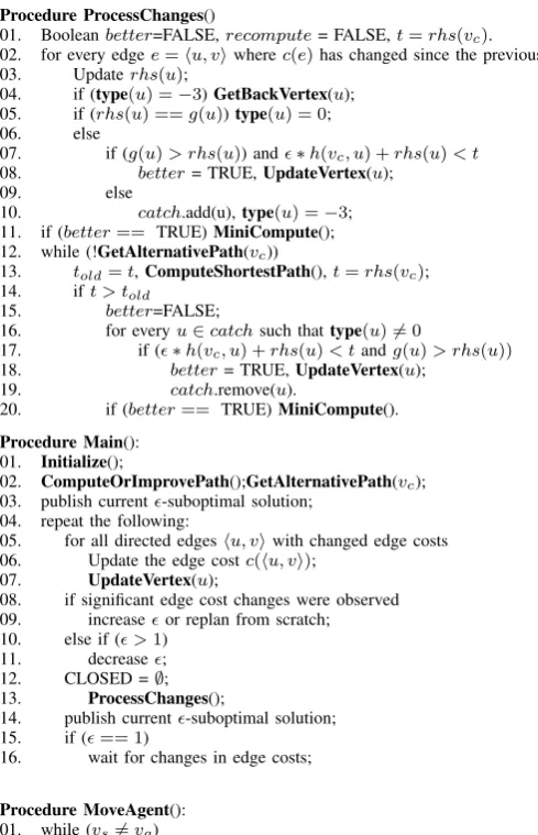
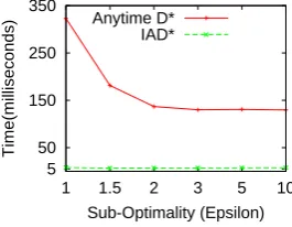
Form Figure 2 to 5, AD* and IAD* are compared on rock-and-garden benchmarks. From Figures 2 to 5, the results of percent = 10 and sensor−radius = 0.1∗size are presented forsize= 300andsize= 500respectively. These figures show the number of heap operations and also the time consumed as a function of sub-optimality EPSILON(ϵ). From the figures, we can see that IAD* gains more than one order of speeding up than AD* in some cases. About the consumed time, IAD* needs extra time to calculate the alternative path besides the time of applying heap operations which is different from AD*. From the figures we can see that in IAD* the time to calculate alternatives cost only takes a very small percentage of the whole time, which means it does not affect the speed of IAD* much. It also shows that heap operations consist the main time complexity in navigation algorithms. Compared with the speeding up of ID* Lite for D* Lite [7], the speed up performance of IAD* for AD* is much better. There are two main reasons, the first one is that there are more alternatives because of sub-optimality. In order to find an alternative of pathP1, in ID* Lite, only pathes with the same cost as P1 can be used as alternatives and there are no pathes with cost smaller than P1. But in IAD*, all pathes with cost ≤ P1 can be used as alternatives. The second one is that AD* needs to reorder its priority queue OPEN every time of recalculating. If IAD* can avoid the recalculating, then the reordering of priority queue can be skipped. The method used in [3] to avoid reordering priority queue can also be used in AD* by modifications introduced in [17]. Unfortunately, the heuristic used in AD* is not consistent, hence that method will cause a lot of reinsertion of key values of vertices because of updating. In [17], the authors choose to reorder the priority queue when recalculating and consider this operation is bearable for time.

The second set of benchmarks, Parking-lot benchmarks, is intended to model agent navigating in the presence of terrain changes. Compared with rock-and-garden benchmarks, we are more interested in parking-lot benchmarks. The reason is the later can simulate the practical environment better. Hence we will give more comparisons between IAD* and AD* on this kind of benchmarks. Terrain changes are commonly encountered by autonomous vehicles of all kinds and may represent the movement of other vehicles and structures in the agent’s environment. A number of tokens equal to a given fixed percentage of vertices are initially created and distributed over vertices in the grid, at most one token

1.0^3 2.0^4 4.0^4 8.0^4 1.2^5

1 1.5 2 3 5 10

Heap Percolations

Sub-Optimality (Epsilon) Anytime D*

[image:4.595.354.497.52.154.2]

IAD*

Fig. 2. size= 300, percent= 10, sensor−radius= 30(rock− and−garden)

2 20 40 80 120

1 1.5 2 3 5 10

Time(milliseconds)

[image:4.595.359.493.195.297.2]

IAD*

covering any vertex. As an agent moves from vertex to vertex through the grid tokens move vertex to vertex as well. Tokens are never destroyed or removed from the grid and the rules for moving tokens do not change: on each round a token on vertexvmoves to a vertex adjacent tov with probability 0.5 and the particular vertex it moves to is determined randomly and uniformly from the set of all adjacent vertices that do not contain a token when the token is moved. Tokens are moved sequentially so there is never more than one token on a vertex. Any vertex covered by a token at any point in the simulation is considered blocked at that point which means all edge costs into the vertex equal ∞. A vertex with no

4.0^3 5.0^4 1.0^5 2.0^5 4.0^5

1 1.5 2 3 5 10

Heap Percolations

IAD*

5 50 150 250 350

1 1.5 2 3 5 10

Time(milliseconds)

IAD*

[image:4.595.354.496.513.614.2] [image:4.595.359.492.654.757.2]

(5)

token is unblocked and edge costs into it are not∞. From Figure 6 to 9, IAD* and AD* are compared similarly as from Figures 2 to 5. We can see that IAD* can also get one order of speeding up, but not as good as in rock-and-garden benchmarks. The reason is that in parking-lot benchmarks, more recalculating are needed by IAD*. This is similar as ID* Lite compared with D* Lite [7]. As we have seen, the time has similar plot as heap percolation, hence below we only show the heap percolation plot because of the limited space.

5.0^3 5.0^4 1.0^5 2.0^5 3.0^5

1 1.5 3 5 10

Heap Percolations

[image:5.595.360.491.52.151.2]

IAD*

Fig. 6. size= 300, percent= 10, sensor−radius= 30(P arking− lot)

10 70 140 280

1 1.5 3 5 10

Time(milliseconds)

[image:5.595.98.241.193.295.2]

IAD*

2.0^4 2.0^5 4.0^5 6.0^5 1.2^6

1 1.5 3 5 10

Heap Percolations

[image:5.595.351.499.194.299.2]

IAD*

In Figures 10 and 11, AD* and IAD* are compared similarly as in Figures 6 and 8, but withpercent= 20. This is to show whether IAD* can perform well in dramatically changing environments. We can see IAD* can still achieve up to one order times of speeding up than AD*. Also, from such figures we can see that the plot of AD* decreases faster than IAD*. Hence we can say that with other conditions made certain, the smaller the sub-optimality required, the better IAD* performs.

20 200 400 600 1100

1 1.5 3 5 10

Time(milliseconds)

IAD*

2.0^4 1.0^5 2.0^5 3.0^5 4.0^5

1 1.5 3 5 10

Heap Percolations

[image:5.595.100.237.354.454.2]

IAD*

Fig. 10. size = 300, percent = 20, sensor − radius = 30(P arking−lot)

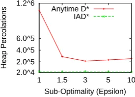
In Figure 12, results are compared with different sensor-radius given size = 300, percent= 3 andϵ = 3. We can see the heap operations increases withsensor−raduis. The reason is that in parking-lot benchmarks the blockages are keeping moving, hence a larger sensor-radius means more changes observed which may cause more updating.

In Figure 13, results are compared with differentpercent given size = 300, sensor−radius = 30 and ϵ = 3. We can see that IAD* has heap operations increased faster than AD* when percent is increased. When percent is increased, in order to find an alternative, more recalculations are needed

1.0^5 3.0^5 8.0^5 1.2^6 1.8^6

1 1.5 3 5 10

Heap Percolations

[image:5.595.100.238.513.612.2]

IAD*

Fig. 11. size = 500, percent = 20, sensor − radius = 50(P arking−lot)

5.0^3 2.5^4 5.0^4 7.5^4 1.0^5

10 15 20 30

Heap Percolations

Radius Anytime D*

[image:5.595.352.497.518.614.2]

IAD*

[image:5.595.350.502.662.765.2]

(6)

in IAD*, which affects its performance. Hence, in parking-lot kind of environments, if the changing of terrain is relatively light, IAD* can have a better performance than in heavily changing environments. From the figure, we can also see that, even with percent= 30, IAD* can still get about two times speeding up than AD*.

5.0^3 2.0^4 5.0^4 8.0^4 1.2^5

10 15 20 30

Heap Percolations

Percent Anytime D*

[image:6.595.98.240.145.246.2]

IAD*

Fig. 13. size= 300, sensor−radius= 30, ϵ= 3(P arking−lot)

At last in Figure 14, results are compared with different sizegivenpercent= 10, sensor−radius= 30andϵ= 3. The results show that IAD* is very scalable in parking-lot benchmarks.

1.0^3 2.0^4 5.0^4 1.0^5 2.0^5

100 200 300 500

Heap Percolations

Percent Anytime D*

IAD*

Fig. 14. percent= 10, sensor−radius= 30, ϵ= 3(P arking−lot)

From the results above, we can see IAD* returns the first qualified sub-optimal path in a shorter time than AD*. Also when other conditions unchanged and in rock-and-garden benchmarksϵfrom1to1.5 IAD* can save about 25 percent of calculations; but in parking-lot benchmarks, the calculations of IAD* varies a little. So IAD* has the ability of returning a high sub-optimal path especially in parking-lot style of environments, and when something emergency happens, for example a lot of changes observed, the first sub-optimal path can be returned fast; after that, IAD* can continue to improve current path until time runs out. I.e., a desired sub-optimal path can be guaranteed to be found in a short time with a high possibility, which also means more time can be used to improve the firstly returned path. Hence, we can conclude that IAD* can return the first sub-optimal path faster than AD* in various random benchmarks, from which IAD* gains a better potentiality to return high sub-optimal path within limited time.

IV. CONCLUSION ANDNEXTSTEP OFWORK

In this paper, we propose a new dynamic anytime al-gorithm IAD*. IAD* improves AD* following the similar strategy as that ID* Lite improves D* Lite. That is, IAD* will try to find an alternative of original path instead of

recalculating immediately as in AD*. Moreover, if an alter-native is not available, in order to avoid a full recalculation IAD* will try to propagate changes part by part with the help of a threshold until a new sub-optimal path found. Experimental results show that IAD* can achieve up to one order of speeding up in various random benchmarks. There is still much work can be done in the next step. For example, We will consider when there is an upper bound of heap operations allowed if there are limited resource and how to make the algorithm to achieve a better sub-optimality; As discussed in this paper IAD* has a better potential to support high sub-optimal path, so we can compare this aspect of AD* and IAD* by experiment; Anytime Weighted A*(AWA*) [8] is demonstrated performing better in some benchmarks to achieve a higher sub-optimality than other algorithms, so combining IAD* with AWA* to get a new faster algorithm is also an interesting work we will do.

Acknowledgement:The work of this paper was supported by the Strategic Priority Research Program of Chinese Academy of Sciences under Grant XDA06010702, the State Key Laboratory of Information Security, Chinese Academy of Sciences, the National Natural Science Foundation of China (Grants 61070172 and 10990011).

REFERENCES

[1] S. Koenig and M. Likhachev, “D*lite,” inEighteenth national confer-ence on Artificial intelligconfer-ence 2002, pp. 476–483.

[2] ——, “Improved fast replanning for robot navigation in unknown terrain,” 2002, pp. 968–975.

[3] A. Stentz, “The focussed d* algorithm for real-time replanning,” in Proceedings of the International Joint Conference on Artificial Intelligence 1995, pp. 1652–1659.

[4] ——, “Optimal and efficient path planning for partially-known en-vironments,” The Kluwer International Series in Engineering and Computer Science, vol. 388, pp. 203–220, 1997.

[5] W. Yue and J. Franco, “Avoiding unnecessary calculations in robot navigation,” in Proceedings of World Congress on Engineering and Computer Science 2009, pp. 718–723.

[6] ——, “A new way to reduce computing in navigation algorithm,”

Journal of Engineering Letters, vol. 18(4), 2010.

[7] W. Yue, J. Franco, W. Cao, and H. Yue, “Id* lite: improved d* lite algorithm,” inProceedings of 26th Symposium On Applied Computing 2011, pp. 1364–1369.

[8] E. A. Hansen and R. Zhou, “The heuristic search under conditions of error,” Journal of Artificial Intelligence Research, vol. 28, pp. 267– 297, 2007.

[9] L. Harris, “The heuristic search under conditions of error,”Artificial Intelligence, vol. 5(3), pp. 217–234, 1974.

[10] R. Zhou and E. Hansen, “Multiple sequence alignment using anytime a*,” inProceedings of Conference on Articial Intelligence 2002, pp. 975–976.

[11] R. Korf, “Linear-space best-first search,”Artificial Intelligence, vol. 62(1), pp. 41–78, 1993.

[12] I. Pohl, “Heuristic search viewed as path finding in a graph,”Artificial Intelligence, vol. 1(3), pp. 193–204, 1970.

[13] H. Davis, A. Bramanti-Gregor, and J. Wang, “The advantages of using depth and breadth components in heuristic search,”Methodologies for Intelligent Systems, vol. 3, pp. 19–28, 1988.

[14] M. Likhachev, G. Gordon, and S. Thrun, “Ara*: anytime a* with provable bounds on sub-optimality,”Advances in Neural Information Processing Systems, 2003.

[15] S. Koenig and M. Likhachev, “Incremental a*,”Advances in Neural Information Processing Systems, pp. 1539–1546, 2002.

[16] S. Koenig, M. Likhachev, and D. Furcy, “Lifelong planning a*,”

Artificial Intelligence Journal, vol. 155(1-2), pp. 93–146, 2004. [17] M. Likhachev, D. Ferguson, G. Gordon, A. Stentz, and S. Thrun,

“Anytime dynamic a*: An anytime, replanning algorithm,” in Pro-ceedings of the International Conference on Automated Planning and Scheduling 2005.

[image:6.595.94.244.348.453.2]